
Short Run Supply Curve of a Firm
Enroll to start learning
You’ve not yet enrolled in this course. Please enroll for free to listen to audio lessons, classroom podcasts and take practice test.
Interactive Audio Lesson
Listen to a student-teacher conversation explaining the topic in a relatable way.
Understanding Supply Curve
🔒 Unlock Audio Lesson
Sign up and enroll to listen to this audio lesson

Today, we will explore how a firm's supply curve is established in a perfectly competitive market. Can anyone tell me what a supply curve represents?

I think it shows the quantity of goods a firm would sell at different prices.
Exactly! The supply curve reflects the quantity supplied at various market prices. It is derived from the firm's marginal cost curve, particularly the rising section of the curve. Now, how do we determine the output level a firm will produce?

Maybe it depends on the price level relative to average variable costs?
Great point! If the market price is higher than the minimum average variable cost, the firm will produce at a profit-maximizing output. Remember the acronym AVC—Average Variable Cost—helps us gauge production viability here.

How do we visualize these price points?
Excellent question! Let's visualize this in our next session. For now, we can conclude that the supply curve indicates quantities produced based on market price.
Price and Output Connections
🔒 Unlock Audio Lesson
Sign up and enroll to listen to this audio lesson

Let's dive deeper into when a firm will choose to produce zero output. Can someone explain when this scenario occurs?

It happens when the market price is less than the minimum AVC!
Exactly! In that case, the firm cannot cover its variable costs, so it would cease production. Let’s also consider the graphical depiction together.
What does that graph look like?
In our graph, the supply curve starts at the price level where AVC reaches its minimum. If the market price falls below that point, the quantity supplied will be zero.
So, the rising section of the marginal cost curve signifies that?
Correct! This section reflects the supply behavior when prices are above average variable costs.
Shifts in Supply Curve
🔒 Unlock Audio Lesson
Sign up and enroll to listen to this audio lesson
Now, let's explore the external factors affecting a firm's supply curve. Can anyone name one?
Technological advancements could lower production costs?
Exactly! Technological progress generally shifts the supply curve to the right, enabling firms to produce more at the same price levels. Anyone know another factor?
What about input prices? If they increase, it raises production costs!
Precisely! Changes in input prices lead to shifts in the supply curve. If costs increase, the curve shifts left, meaning firms supply less at every price.
So, more costs mean less supply. Got it!
Remember, staying alert to these shifts will help you understand market dynamics more thoroughly. Great job everyone!
Introduction & Overview
Read summaries of the section's main ideas at different levels of detail.
Quick Overview
Standard
In this section, we explore how a firm determines its output in the short run under perfect competition. We analyze how the firm's supply curve is derived from its marginal cost curve and what conditions influence its output decision based on market prices.
Detailed
In perfect competition, a firm's short-run supply curve is derived from its marginal cost (MC) structure and average variable cost (AVC) conditions. This section outlines two cases based on market price relative to minimum AVC: (1) when the market price is greater than or equal to the minimum AVC, leading firms to produce a profit-maximizing output, and (2) when the market price is less than the minimum AVC, resulting in zero output production. The derivation of the supply curve illustrates how it is shaped by the rising portion of the marginal cost curve and indicates the firm's willingness to supply at various price levels. Additionally, the behavior surrounding firm responses to market prices, conditions for stopping production, and factors like technological progress and changes in input prices are discussed.
Youtube Videos


Audio Book
Dive deep into the subject with an immersive audiobook experience.
Case 1: Price is Greater Than or Equal to Minimum AVC
Chapter 1 of 3
🔒 Unlock Audio Chapter
Sign up and enroll to access the full audio experience
Chapter Content
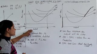
Suppose the market price is p₁, which exceeds the minimum AVC. We start out by equating p with SMC on the rising part of the SMC curve; this leads to the output level q₁. Note also that the AVC at q₁ does not exceed the market price, p₁. Thus, all three conditions highlighted in section 3 are satisfied at q₁. Hence, when the market price is p₁, the firm’s output level in the short run is equal to q₁.
Detailed Explanation
In this case, we consider when the market price is equal to or higher than the minimum average variable cost (AVC). The firm will choose to produce because the price they receive for their product is high enough to cover their variable costs. By equating the price (p₁) with the short-run marginal cost (SMC) of production, we determine the profit-maximizing output level, designated as q₁. Since the price is higher than the average variable cost at this output level, the firm can operate profitably.
Examples & Analogies
Imagine a lemonade stand. If the price a customer is willing to pay for a glass of lemonade is greater than the cost of the lemons, sugar, and cups (average variable cost), the stand will continue to sell lemonade. For example, if selling lemonade costs 50 cents per glass but the market price is $1, the stand will produce as many glasses as they can sell at this price.
Case 2: Price is Less Than the Minimum AVC
Chapter 2 of 3
🔒 Unlock Audio Chapter
Sign up and enroll to access the full audio experience
Chapter Content
Suppose the market price is p₂, which is less than the minimum AVC. We have argued (see condition 3 in section 3) that if a profit-maximising firm produces a positive output in the short run, then the market price, p₂, must be greater than or equal to the AVC at that output level. But notice from Figure 4.7 that for all positive output levels, AVC strictly exceeds p₂. In other words, it cannot be the case that the firm supplies a positive output. So, if the market price is p₂, the firm produces zero output.
Detailed Explanation
In this scenario, the market price is lower than the minimum average variable cost. Since the revenue from selling the product wouldn't even cover the variable costs of production, the firm cannot profitably produce any output. Therefore, the firm decides to shut down temporarily, and the output level remains at zero. This ensures that the firm does not incur losses from producing more than it can sell profitably.
Examples & Analogies
Using the lemonade stand again, suppose the price customers are willing to pay drops to 25 cents while it still costs the stand 50 cents to make a glass. Since selling lemonade at this price means losing money, the stand will close until prices rise to ensure they don't incur losses.
Conclusion: The Short Run Supply Curve
Chapter 3 of 3
🔒 Unlock Audio Chapter
Sign up and enroll to access the full audio experience
Chapter Content
Combining cases 1 and 2, we reach an important conclusion. A firm’s short run supply curve is based on its short run marginal cost curve (SMC) and the average variable cost curve (AVC). It is represented from and above the minimum AVC together with zero output for all prices strictly less than the minimum AVC.
Detailed Explanation
The short run supply curve shows the relationship between market prices and the quantity a firm is willing to supply at those prices under short-run conditions. If market prices are above the minimum AVC, the firm supplies a positive output corresponding to its marginal cost. However, if market prices fall below this threshold, the firm does not produce at all because it cannot cover its variable costs.
Examples & Analogies
Think of a baker who sells cakes. If they can sell cakes for $20 each and it costs them $10 in ingredients and labor (AVC) to make one cake, they will produce cakes. But if the price falls to $5, they won’t bake any cakes since they would lose $5 on each one sold. The short run supply curve captures this behavior: they will only supply cakes at prices that cover their costs.
Key Concepts
-
Short Run Supply Curve: Represents how much a firm will produce at different price levels in the short run.
-
Marginal Cost Curve: The cost of producing one additional unit, which determines the supply curve.
-
Average Variable Cost: The lowest price at which a firm can produce without incurring losses in the short run.
Examples & Applications
If a candle manufacturer produces and sells 2 boxes of candles at a price of Rs 10, its total revenue would be Rs 20, providing a basis for analyzing supply decisions.
In perfect competition, if input costs rise and push marginal costs higher, the firm’s supply curve will shift to the left, meaning less quantity supplied at any given price.
Memory Aids
Interactive tools to help you remember key concepts
Rhymes
When AVC runs high, production is shy, stop the flow, it's goodbye!
Stories
Imagine a candle maker who can only sell candles if the price covers more than just the wax! If the market dips, it’s economic bliss to quit making candles altogether!
Memory Tools
Remember 'PEAR' for the factors impacting supply: Price, Entry conditions, Average costs, and Resource prices.
Acronyms
COST for remembering conditions
Costs must be covered
Output is related
Supply decisions are based on
Technology matters.
Flash Cards
Glossary
- Supply Curve
A graph showing the relationship between the price of a good and the quantity that suppliers are willing to sell.
- Marginal Cost (MC)
The additional cost incurred from producing one more unit of a good.
- Average Variable Cost (AVC)
Total variable costs divided by the quantity of output produced.
- ProfitMaximizing Output
The level of output that maximizes a firm's profit, found where marginal revenue equals marginal cost.
Reference links
Supplementary resources to enhance your learning experience.