
Supply Curve of a Firm
Enroll to start learning
You’ve not yet enrolled in this course. Please enroll for free to listen to audio lessons, classroom podcasts and take practice test.
Interactive Audio Lesson
Listen to a student-teacher conversation explaining the topic in a relatable way.
Understanding Supply Curves
🔒 Unlock Audio Lesson
Sign up and enroll to listen to this audio lesson

Today, we will learn about the supply curve of a firm. Can anyone tell me what a supply curve represents?

Is it the relationship between the price of the good and the quantity supplied?
Exactly! The supply curve demonstrates how much of a product a firm is willing to sell at various prices. It's essential in understanding market behavior.

Is the supply curve the same in the short run and the long run?
Great question! No, it's not the same. In the short run, we look at the rising part of the short-run marginal cost curve, while the long-run supply curve is tied to long-run marginal costs. Remember this as 'SRMC for the Short Run' and 'LRMC for the Long Run'!
Short Run vs. Long Run Supply
🔒 Unlock Audio Lesson
Sign up and enroll to listen to this audio lesson

Now, let's explore how a firm's supply decisions differ in the short run versus the long run.

So does the firm's output depend on market price in both cases?
Absolutely! When the market price is above the minimum average variable cost (AVC), the firm will produce, and output increases as prices rise.

What happens below that price?
Good observation. If the price falls below the minimum AVC, the firm will not produce, and we denote that point as the shut-down point. This is very significant for firms' survival in competitive markets.
Factors Affecting Supply Curve
🔒 Unlock Audio Lesson
Sign up and enroll to listen to this audio lesson
Various factors influence the supply curve, such as technological advancement and input prices.
How does technology impact supply?
When technology improves, firms can produce more efficiently, thus shifting their supply curve to the right. Remember, 'Tech makes it better, Supply gets lighter!'
What about when input prices increase?
In that case, costs go up, leading to a leftward shift in the supply curve. So when costs rise, 'Supply drops, while cost hops!'
Impact of Taxes on Supply
🔒 Unlock Audio Lesson
Sign up and enroll to listen to this audio lesson
Another important factor is taxes; how do you think taxes affect supply?
I think if the government imposes a tax, it increases costs for firms.
Exactly! A unit tax shifts the supply curve to the left because it increases average and marginal costs.
So firms will supply less at each price point?
Correct! This ties back to our earlier discussion: higher costs generally mean lower supply.
Market Supply vs. Firm Supply
🔒 Unlock Audio Lesson
Sign up and enroll to listen to this audio lesson
Lastly, let's talk about how individual supply curves combine to form the market supply curve.
Is it just the sum of all individual firms’ supplies?
Correct! It’s a horizontal summation of all firms' supply at a given price. Think 'All firms unite for market supply!'
Does that mean if more firms enter the market, the supply curve would shift?
Indeed! More firms in a market usually mean more supply. Remember, 'More firms, more goods from the storms!'
Introduction & Overview
Read summaries of the section's main ideas at different levels of detail.
Quick Overview
Standard
The supply curve of a firm illustrates the quantity of goods a firm is willing to supply at different market prices, accounting for both short-run and long-run considerations. It elaborates on the conditions under which a firm maximizes profit and how changes in the market affect its supply decisions.
Detailed
In Chapter 4.4, we delve into the nature of the supply curve of a firm within a perfectly competitive market. The supply curve represents the quantity of output a firm is willing to sell at different market prices, assuming that technology and factor prices remain stable. We differentiate between the short-run and long-run supply curves, elaborating on how the firm's profit-maximizing output is derived from its marginal cost structure. In the short run, the supply curve is driven by the firm's short-run marginal cost curve, whereas the long run supply curve is contingent on the long-run marginal cost structure. Key conditions such as the relationship between market price and average/marginal cost are essential for understanding the firm's supply behavior. The section also covers the implications of technological changes and input price fluctuations on the supply curve, leading to crucial insights on market dynamics.
Youtube Videos


Audio Book
Dive deep into the subject with an immersive audiobook experience.
Definition of Supply and Supply Schedule
Chapter 1 of 5
🔒 Unlock Audio Chapter
Sign up and enroll to access the full audio experience
Chapter Content
A firm’s ‘supply’ is the quantity that it chooses to sell at a given price, given technology, and given the prices of factors of production. A table describing the quantities sold by a firm at various prices, technology and prices of factors remaining unchanged, is called a supply schedule. We may also represent the information as a graph, called a supply curve.
Detailed Explanation
The supply of a firm refers to the quantity of products it is prepared to sell at varying price levels, while assuming that factors such as technology and production costs are static. The supply schedule is essentially a table that outlines the quantities that a firm can sell at different prices, demonstrating the firm’s response to price changes. This table can be transformed into a visual representation known as a supply curve, which graphically shows the relationship between price and quantity supplied.
Examples & Analogies
Think about a lemonade stand on a hot day. The owner of the stand will decide how many cups of lemonade to sell based on how much they can charge for each cup. If they know they can sell 50 cups at $1 each, but only 30 cups at $0.50 each, this information can be organized into a supply schedule or graph to show how quantity changes with prices.
Short Run Supply Curve
Chapter 2 of 5
🔒 Unlock Audio Chapter
Sign up and enroll to access the full audio experience
Chapter Content
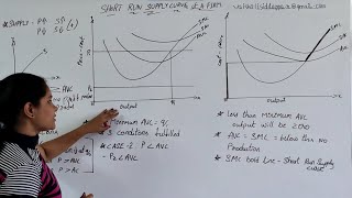
We distinguish between the short run supply curve and the long run supply curve. Let us turn to Figure 4.7 and derive a firm’s short run supply curve. We shall split this derivation into two parts. We first determine a firm’s profit-maximising output level when the market price is greater than or equal to the minimum AVC. This done, we determine the firm’s profit-maximising output level when the market price is less than the minimum AVC.
Detailed Explanation
The short run supply curve illustrates how a firm's output levels change with varying market prices, taking certain conditions into account. First, if the market price is above a specific average variable cost (AVC), the firm will produce a level of output that maximizes profit. Conversely, if the market price is below this minimum AVC, the firm will not produce any output since it cannot cover variable costs. Thus, the short run supply curve is formed from the rising portion of the marginal cost curve above this AVC threshold, while for prices below this threshold, the output remains zero.
Examples & Analogies
Imagine the lemonade stand again. On a day when the price of lemonade is $1, the stand might sell many cups. However, if the price falls to $0.25, the seller might find that the costs of making lemonade (like buying lemons and sugar) mean it's not worth selling any at this low price. Therefore, they will only sell lemonade when they can at least cover those costs.
Long Run Supply Curve
Chapter 3 of 5
🔒 Unlock Audio Chapter
Sign up and enroll to access the full audio experience
Chapter Content
We may also examine the long run supply curve of a firm. Similar to the short run, we can derive the long run supply curve by considering two cases based on the market price relative to average costs. Case 1: Price greater than or equal to the minimum (long run) AC. Case 2: Price less than the minimum (long run) AC.
Detailed Explanation
The long run supply curve is derived by analyzing how a firm's output adjusts to changes in market prices when all production factors can be varied. If the market price is above the long-run average cost (LRAC) of production, the firm will produce at the quantity that maximizes profit where the price equals long-run marginal cost (LRMC). However, if the market price falls below the minimum LRAC, the firm will not produce at all in the long run, as it would not be able to cover its average costs, leading to zero supply at those price levels.
Examples & Analogies
Consider a factory that produces furniture. If the market price for chairs rises above the cost of materials and labor for making them, the factory will increase production to take advantage of the higher prices. But if prices fall below what it costs to produce even one chair, the factory would choose to stop production altogether until prices improve.
Shut Down Point
Chapter 4 of 5
🔒 Unlock Audio Chapter
Sign up and enroll to access the full audio experience
Chapter Content
Along the supply curve, the last price-output combination at which the firm produces positive output is the point of minimum AVC where the SMC curve cuts the AVC curve. Below this, there will be no production. This point is called the short run shut down point of the firm.
Detailed Explanation
The shut down point is the minimum average variable cost at which a firm can continue operating. When prices fall below this point, the firm is unable to cover its variable costs, leading it to cease operations. The interaction of the short run marginal cost curve (SMC) with the average variable cost curve provides this critical insight into determining if a firm should continue to produce or shut down temporarily.
Examples & Analogies
Imagine a local coffee shop that brews its drinks at a cost of $3 each, covering its ingredients and worker wages. If customers are only willing to pay $2 for a cup, the shop realizes that it will not cover production costs and might choose to close the shop until prices rise enough to cover its costs.
Normal Profit and Break-even Point
Chapter 5 of 5
🔒 Unlock Audio Chapter
Sign up and enroll to access the full audio experience
Chapter Content
The minimum level of profit that is needed to keep a firm in the existing business is defined as normal profit. A firm that does not make normal profits is not going to continue in business. Normal profits are therefore a part of the firm’s total costs.
Detailed Explanation
Normal profit is essentially the minimum compensation required to keep a firm operating and in the market. It is considered an opportunity cost, reflecting the earnings a firm could generate from alternative ventures. When a firm's profits exceed this threshold, it earns super-normal profits. The break-even point is identified on the supply curve where the firm earns just enough revenue to cover its costs - no profit and no loss.
Examples & Analogies
Think of a person running a food truck. They need to make at least $100 a day to cover costs like food, fuel, and permits. Anything less, they operate at a loss. If they make this $100 (normal profit), they're breaking even. If they make $120, they're generating extra income (super-normal profit), and if they drop to $80, they might consider closing the food truck entirely.
Key Concepts
-
Supply Curve: A graphical representation that shows the quantity supplied at various price levels.
-
Short Run Supply Curve: Relates to how a firm adjusts production with a fixed-input setup.
-
Long Run Supply Curve: Derives from the firm's ability to adjust all factors of production.
-
Shut Down Point: The critical price level below which production ceases.
-
Normal Profit: The minimum profit necessary for continued business operations.
Examples & Applications
If a firm finds that the market price of its product rises, it may increase output according to the upward slope of its supply curve.
A tech company that innovates its production process may lower production costs, shifting its supply curve to the right.
Memory Aids
Interactive tools to help you remember key concepts
Rhymes
When prices climb, output will rise; that's how the supply curve lies!
Stories
Imagine a lemonade stand. When prices go up, the stand owner decides to squeeze more lemons to earn more money.
Memory Tools
Remember 'SRMC' for Short Run Marginal Cost aids in drawing your supply curve.
Acronyms
SUPPLY = Short-run, Upward slope, Prices lead to more output, Low costs, Yield greater profits.
Flash Cards
Glossary
- Supply Curve
A graphical representation of the relationship between the price of a good and the quantity supplied.
- Short Run Supply Curve
The part of the marginal cost curve that indicates the quantity a firm is willing to supply at different prices, assuming some factors are fixed.
- Long Run Supply Curve
The part of the marginal cost curve that reflects the quantities supplied as all factors can be varied in the long run.
- Shut Down Point
The price level at which a firm chooses to produce no output; occurs when the price is less than the minimum average variable cost.
- Normal Profit
The minimum amount of profit necessary for a company to remain competitive in the market.
- Breakeven Point
The price point at which total revenue equals total cost, resulting in no profit or loss.
Reference links
Supplementary resources to enhance your learning experience.