
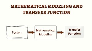
General Procedure for Deriving Transfer Functions
Enroll to start learning
You’ve not yet enrolled in this course. Please enroll for free to listen to audio lessons, classroom podcasts and take practice test.
Interactive Audio Lesson
Listen to a student-teacher conversation explaining the topic in a relatable way.
Modeling a Dynamic System
🔒 Unlock Audio Lesson
Sign up and enroll to listen to this audio lesson

To start deriving a transfer function, we need to model our dynamic system using physical principles. Can anyone remind me what modeling involves?

It involves understanding the physical components and laws governing the system, like Newton's laws for mechanical systems.
Exactly! We also consider Kirchhoff's laws for electrical systems. This leads us to step two, where we write the differential equation based on that model. What do we think is the importance of this equation?

I believe it describes how the system behaves over time?
Right! Remember, the behavior over time is crucial for our analysis. What comes next after writing the differential equation?

We take the Laplace transform of that equation, right?
Correct! Now, let’s summarize our first key points: modeling involves understanding the components and formulating a differential equation to represent system dynamics.
Laplace Transform
🔒 Unlock Audio Lesson
Sign up and enroll to listen to this audio lesson

Now let’s discuss the Laplace transform. Why is it necessary to apply it to our differential equations when deriving transfer functions?

It converts differential equations into algebraic equations, making them easier to handle!
Exactly! And what do we obtain as a result of applying the Laplace transform?
We get an equation in terms of the transformed variables, right?
Yes! And this is essential for isolating our output variable. What’s the next step after this?
We solve for the output in terms of the input.
Correct! So make sure to remember: the Laplace transform simplifies our analysis of dynamic systems significantly!
Deriving Transfer Functions
🔒 Unlock Audio Lesson
Sign up and enroll to listen to this audio lesson
Let’s wrap it up with the final steps. After obtaining the relation between output and input, how do we simplify it to get our transfer function?
We need to rearrange the equation to express the output over the input, right?
Yes! Which brings us to the definition of the transfer function itself. What do we mean by that?
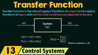
The transfer function is the ratio of the Laplace transform of the output to that of the input!
Great job! And remember, the transfer function gives us significant insights into system dynamics, such as stability and frequency response.
Introduction & Overview
Read summaries of the section's main ideas at different levels of detail.
Quick Overview
Standard
The section details a five-step process for deriving transfer functions from dynamic systems, emphasizing the importance of modeling, formulating differential equations, applying the Laplace transform, and ultimately simplifying the results to establish the relationship between input and output.
Detailed
In this section, we focus on the general procedure for deriving transfer functions essential for analyzing dynamic systems. Transfer functions, which encapsulate the relationship between input and output in a Laplace domain, are derived through a systematic approach outlined in five clear steps:
- Model the System: Use physical principles such as Newton's or Kirchhoff’s laws to create a mathematical model.
- Write the Differential Equation: Formulate the governing differential equation that characterizes the system's dynamics.
- Take the Laplace Transform: Convert the differential equation into the Laplace domain, facilitating the analysis of the system's behavior under various conditions.
- Solve for Output: Rearrange the transformed equation to express the output variable in terms of the input variable.
- Simplify to Get the Transfer Function: Finally, derive the transfer function as the ratio of the Laplace transforms of the output and input, which describes the system’s dynamic response in relation to external influences. This process is crucial for engineers and researchers, enabling a deeper understanding of systems in control engineering and related disciplines.
Youtube Videos

Audio Book
Dive deep into the subject with an immersive audiobook experience.
Step 1: Model the System
Chapter 1 of 5
🔒 Unlock Audio Chapter
Sign up and enroll to access the full audio experience
Chapter Content
- Model the system using physical principles (Newton's law, Kirchhoff’s law, etc.).
Detailed Explanation
In this first step, we start by understanding the dynamic system we want to analyze. This involves using relevant physical laws—like Newton's law for mechanical systems or Kirchhoff’s law for electrical circuits—to create a model that accurately represents how the system behaves. This modeling is crucial because it lays the foundation for deriving the differential equations that describe the system.
Examples & Analogies
Imagine building a bridge, where you must understand the forces acting on it—gravity pulling down, wind pushing against it—using the relevant principles from physics to effectively design a stable structure. Similarly, in system modeling, you're establishing a groundwork based on laws of nature that govern the dynamics of your system.
Step 2: Write the Differential Equation
Chapter 2 of 5
🔒 Unlock Audio Chapter
Sign up and enroll to access the full audio experience
Chapter Content
- Write the differential equation that governs the system’s behavior.
Detailed Explanation
Once we have modeled the system, the next step is to represent its behavior using a differential equation. This equation captures the relationship between the input, output, and various state variables of the system, illustrating how they change over time. For instance, in a mass-spring-damper system, the forces acting on the mass lead directly to an equation relating acceleration to applied forces.
Examples & Analogies
Think of this step like writing the rules for a game. Just as you need a clear set of rules to understand how players, points, and outcomes interact, the differential equation serves as a rule book for the dynamic system, specifying how inputs affect outputs.
Step 3: Take the Laplace Transform
Chapter 3 of 5
🔒 Unlock Audio Chapter
Sign up and enroll to access the full audio experience
Chapter Content
- Take the Laplace transform of the differential equation.
Detailed Explanation
The next step is to apply the Laplace transform to the differential equation. This transforms the time-domain equation into the frequency domain, which simplifies the analysis, especially for linear time-invariant (LTI) systems. Using the Laplace transform allows us to work with algebraic equations instead of differential equations, making it easier to manipulate and solve.
Examples & Analogies
Consider using a tool to convert currency values instantly. Just as a currency converter gives you a new numerical representation that is easier to work with, the Laplace transform provides a mathematical tool to transform complicated time-domain equations into a more manageable form.
Step 4: Solve for the Output
Chapter 4 of 5
🔒 Unlock Audio Chapter
Sign up and enroll to access the full audio experience
Chapter Content
- Solve for the output in terms of the input.
Detailed Explanation
After taking the Laplace transform, the next objective is to isolate the output variable in the transformed equation. This means expressing the output as a function of the input, enabling us to understand how the system will respond to any given signal. This step often involves rearranging terms and simplifying the equation to express output clearly.
Examples & Analogies
Imagine a recipe where you have all ingredients but need to know how much cake you’ll get based on the quality and quantity of those ingredients. Solving for output in this step allows us to predict the outcome of our dynamic system when different input signals are applied.
Step 5: Simplify to Get the Transfer Function
Chapter 5 of 5
🔒 Unlock Audio Chapter
Sign up and enroll to access the full audio experience
Chapter Content
- Simplify to get the transfer function (i.e., the ratio of the Laplace transforms of the output and input).
Detailed Explanation
In the final step, we derive the transfer function by taking the ratio of the Laplace transform of the output to that of the input. This transfer function is a key descriptor of the system as it encapsulates the system’s dynamic behavior in relation to the input and output. It helps in analyzing various properties like stability and response to different inputs.
Examples & Analogies
Think of this step like distilling a complex story down to a simple summary. Just as a summary captures the essence of a narrative, the transfer function summarizes the system's behavior in a concise mathematical form, making it easier to predict how the system will act under various input conditions.
Key Concepts
-
Modeling: The process of creating a mathematical representation of a dynamic system using physical laws.
-
Differential Equation: Represents the system dynamics and relates variables to their rates of change.
-
Laplace Transform: A tool that simplifies the analysis of differential equations by converting them into algebraic forms.
-
Transfer Function: The resultant mathematical expression that defines the relationship between input and output in the Laplace domain.
Examples & Applications
For a mass-spring-damper system, the differential equation can be derived using Newton's laws, leading to a transfer function that describes the system's behavior under external force.
In electrical engineering, the transfer function of a series RLC circuit can be derived through Kirchhoff's laws, illustrating the relationship between voltage and current.
Memory Aids
Interactive tools to help you remember key concepts
Rhymes
Model, solve, transform with glee, ratio of output, input, you'll see!
Stories
Once in a lab, a teacher showed students how modeling a mechanical system led to writing equations, transforming them for clarity, and finally deriving a guiding formula for their dynamic world - the transfer function!
Memory Tools
Remember MLT for deriving transfer functions: Model, Laplace, Transform.
Acronyms
To remember the process
MDSST - Model
Differential Equation
Solve for Output
Simplify to get Transfer Function.
Flash Cards
Glossary
- Transfer Function
A mathematical representation that describes the relationship between the input and output of a linear time-invariant system in the Laplace domain.
- Differential Equation
An equation that relates a function with its derivatives, used to describe dynamic systems.
- Laplace Transform
A mathematical operation that converts functions of time into functions of complex frequency, facilitating the analysis of linear time-invariant systems.
- Dynamic System
A system that changes over time in response to inputs, typically described by differential equations.
Reference links
Supplementary resources to enhance your learning experience.