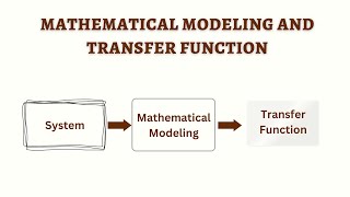
In control systems engineering, dynamic systems refer to systems that change over time in response to inputs. These systems are described by differential equations that represent their physical, mechanical, electrical, or other dynamic processes. To analyze and design control systems, we often need to convert these time-domain equations into the frequency domain using transfer functions.

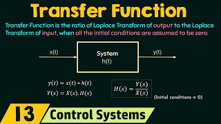
A transfer function (TF) is a mathematical representation of the relationship between the input and output of a linear time-invariant (LTI) system, expressed in the Laplace domain.

A dynamic system is typically modeled based on its physical components, such as masses, springs, dampers (mechanical systems), or resistors, capacitors, and inductors (electrical systems). These systems are governed by differential equations that describe their behavior over time.

Basic Types of Dynamic Systems:
1. Mechanical Systems:
- Mass-Spring-Damper System
- Rotational Systems
2. Electrical Systems:
- RLC Circuits (Resistor, Inductor, Capacitor)
- Electric Motors
3. Fluid Systems:
- Tanks, Pumps, Valves, etc.
4. Thermal Systems:
- Heat exchangers, furnaces, and temperature-controlled systems.

Let’s begin with one of the simplest examples of a mechanical system: a Mass-Spring-Damper system.

System Description:
- Mass (m): The object that moves in response to forces.
- Spring constant (k): Represents the elasticity of the spring.
- Damping coefficient (b): Accounts for the frictional force opposing motion.

In such a system, the force applied to the mass causes it to move, and this movement can be modeled by Newton’s Second Law of Motion:
F(t)=ma(t)
where a(t) is the acceleration of the mass and F(t) is the applied force.

For the spring and damper, the forces are given by:
- Spring force: Fspring=−kx(t)
- Damping force: Fdamper=−b(dx(t)/dt)

where x(t) is the displacement of the mass.

Equation of Motion:
The total force on the mass is the sum of the applied force, the spring force, and the damping force. According to Newton's second law:
ma(t)=Fapplied−Fspring−Fdamper
Substituting the expressions for the spring and damping forces:
m(d^2x(t)/dt^2)=Fapplied(t)−kx(t)−b(dx(t)/dt)
Rearranging this:
m(d^2x(t)/dt^2)+b(dx(t)/dt)+kx(t)=Fapplied(t)
This is the differential equation that governs the motion of the mass. It is a second-order differential equation.

To analyze this system in the Laplace domain (frequency domain), we convert the differential equation into its Laplace form. First, recall that:
L{dnx(t)dtn}=snX(s)−sn−1x(0)−sn−2(dx(0)/dt)−⋯
For the second-order mass-spring-damper system, the Laplace transform of the equation is:
ms^2X(s)+bsX(s)+kX(s)=Fapplied(s)
Factoring out X(s):
X(s)(ms^2+bs+k)=Fapplied(s)
The transfer function (TF) G(s) is defined as the ratio of the output X(s) to the input Fapplied(s):
G(s)=X(s)/Fapplied(s)=1/(ms^2+bs+k).
This is the transfer function of the mass-spring-damper system.

To derive the transfer function for any dynamic system, follow these steps:
1. Model the system using physical principles (Newton's law, Kirchhoff’s law, etc.).
2. Write the differential equation that governs the system’s behavior.
3. Take the Laplace transform of the differential equation.
4. Solve for the output in terms of the input.
5. Simplify to get the transfer function (i.e., the ratio of the Laplace transforms of the output and input).

The transfer function provides critical insights into the system's:
- Stability: By analyzing the poles and zeros of the transfer function, we can determine if the system is stable.
- Frequency response: The transfer function can be used to derive frequency-domain analysis techniques, such as Bode plots and Nyquist plots.
- System behavior: The transfer function relates system parameters to the system’s dynamic behavior, allowing us to design controllers that meet specific performance criteria.

In this chapter, we learned how to model dynamic systems from first principles and derive transfer functions. A transfer function is a powerful tool for analyzing and designing control systems, as it represents the relationship between input and output in the Laplace domain. Whether for mechanical, electrical, or other types of systems, deriving transfer functions is essential for predicting system behavior and designing controllers that ensure stability and performance.