
Transfer Function Derivation
Enroll to start learning
You’ve not yet enrolled in this course. Please enroll for free to listen to audio lessons, classroom podcasts and take practice test.
Interactive Audio Lesson
Listen to a student-teacher conversation explaining the topic in a relatable way.
Introduction to Transfer Functions
🔒 Unlock Audio Lesson
Sign up and enroll to listen to this audio lesson

Today, we will explore transfer functions and why they are critical in control systems. Can anyone tell me what a transfer function is?

Is it the relationship between input and output of a system?
Exactly! It's a mathematical representation in the Laplace domain. Now, what do we need to establish this relationship?

We need a differential equation that describes the system!
Correct! Always start with modeling the physical system using principles like Newton's law or Kirchhoff’s law.

Once we have the differential equation, do we just convert it to the Laplace domain?
Yes! That's a key step. Let's summarize: The transfer function relates input to output and requires a proper differential equation as a starting point.
Laplace Transform of Motion Equation
🔒 Unlock Audio Lesson
Sign up and enroll to listen to this audio lesson

Now, let's proceed with the mass-spring-damper system. We start with the motion equation: what do we remember from Newton's second law?
The force equals mass times acceleration, right?
Correct! The equation: $m \frac{d^2x(t)}{dt^2} + b \frac{dx(t)}{dt} + kx(t) = F_{applied}(t)$ captures that. Now, who can tell me how we transform this to Laplace?

We apply the Laplace transform to each term!
Excellent! We arrive at $ms^2X(s) + bsX(s) + kX(s) = F_{applied}(s)$. What’s our next step?
We can factor out $X(s)$!
Exactly! This allows us to express the relationship clearly, linking our output and input in the Laplace domain.
Deriving the Transfer Function
🔒 Unlock Audio Lesson
Sign up and enroll to listen to this audio lesson
We have $X(s)(ms^2 + bs + k) = F_{applied}(s)$. How do we derive the transfer function?
By isolating $X(s)$ on one side.
Good! From this, we define the transfer function as $G(s) = \frac{X(s)}{F_{applied}(s)} = \frac{1}{ms^2 + bs + k}$. Does anyone know why this form is useful?
It helps in analyzing the system’s stability and behavior!
Right! The poles and zeros can reveal a lot about the system dynamics.
So, we use transfer functions for designing controllers that will stabilize the system?
Exactly! This is why understanding transfer functions is essential in control engineering.
Introduction & Overview
Read summaries of the section's main ideas at different levels of detail.
Quick Overview
Standard
The derivation of the transfer function is crucial for analyzing dynamic systems. This section illustrates the process by transforming the differential equation of a mass-spring-damper system into its Laplace form and extracting the transfer function that relates output to input.
Detailed
Transfer Function Derivation
In this section, we delve into the derivation of the transfer function (TF) for a mass-spring-damper system, a crucial element in control system dynamics. The transfer function expresses the relationship between the output and input in the frequency (Laplace) domain, providing insights into system behavior. Following Newton's Second Law of Motion, we start by formulating the second-order differential equation governing the mass's motion.
Key Steps in Derivation
- Starting with Newton's Law:
The equation of motion is written as:
$$m \frac{d^2x(t)}{dt^2} + b \frac{dx(t)}{dt} + kx(t) = F_{applied}(t)$$
This represents the forces acting on the mass due to the applied force, the spring, and the damper.
- Laplace Transform:
By applying the Laplace transform, we transition to the frequency domain:
$$ms^2X(s) + bsX(s) + kX(s) = F_{applied}(s)$$
- Factoring and Isolation:
Rearranging the equation allows us to express the input-output relationship in Laplace terms:
$$X(s)(ms^2 + bs + k) = F_{applied}(s)$$
- Transfer Function Definition:
The transfer function, defined as the ratio of output to input, is given by:
$$G(s) = \frac{X(s)}{F_{applied}(s)} = \frac{1}{ms^2 + bs + k}$$
Significance
This transfer function provides an avenue for analyzing system properties—including stability and response characteristics—crucial for the design and control of dynamic systems.
Youtube Videos

Audio Book
Dive deep into the subject with an immersive audiobook experience.
Introduction to Laplace Transform
Chapter 1 of 3
🔒 Unlock Audio Chapter
Sign up and enroll to access the full audio experience
Chapter Content
To analyze this system in the Laplace domain (frequency domain), we convert the differential equation into its Laplace form. First, recall that:
L{dnx(t)dtn}=snX(s)−sn−1x(0)−sn−2dx(0)dt−⋯\mathcal{L}\left\{ \frac{d^n x(t)}{dt^n} \right\} = s^n X(s) - s^{n-1} x(0) - s^{n-2} \frac{dx(0)}{dt} - \cdots
Detailed Explanation
The Laplace transform is a powerful mathematical tool used to convert time-domain equations (like differential equations) into the frequency domain. It allows us to work with algebraic equations instead of complex differential equations. The formula indicates that when we take the Laplace transform of the n-th derivative of a function x(t), we get a combination of s, which is a complex frequency variable, and the initial conditions of the function (like its value and its first derivative at time zero). This foundational step is crucial as it translates the dynamics of a system into a format (Laplace domain) where they are easier to manipulate and analyze, especially for control systems.
Examples & Analogies
Imagine translating a complex recipe that requires various timing elements into a checklist format. In this analogy, the original recipe represents the time-domain differential equations, while the checklist symbolizes the Laplace transform—the checklist makes it easier to see what steps (equations) you need to perform without worrying about the timing of actions.
Applying the Laplace Transform to the Mass-Spring-Damper System
Chapter 2 of 3
🔒 Unlock Audio Chapter
Sign up and enroll to access the full audio experience
Chapter Content
For the second-order mass-spring-damper system, the Laplace transform of the equation is:
ms2X(s)+bsX(s)+kX(s)=Fapplied(s)ms^2 X(s) + bsX(s) + kX(s) = F_{\text{applied}}(s)
Detailed Explanation
When applying the Laplace transform to the governing differential equation of the mass-spring-damper system, we transform every term involving derivatives into algebraic terms in the Laplace domain. The output X(s) of the system, which represents the system's response, is affected by the system's properties (mass 'm', damping 'b', and spring constant 'k') and the applied force. This equation represents a typical transfer function formulation in control systems, allowing us to analyze the behavior of our dynamical system in a more manageable form.
Examples & Analogies
Think of it as taking a live concert performance (the time-domain) and recording it to produce a music track (the Laplace domain). During the recording, all the audio components (instruments and voices) are combined into a single track that can be analyzed and edited, much like combining the components of a dynamic system into a formula that you can study and manipulate.
Factoring and Defining the Transfer Function
Chapter 3 of 3
🔒 Unlock Audio Chapter
Sign up and enroll to access the full audio experience
Chapter Content
Factoring out X(s)X(s):
X(s)(ms2+bs+k)=Fapplied(s)X(s) (ms^2 + bs + k) = F_{\text{applied}}(s)
The transfer function (TF) G(s)G(s) is defined as the ratio of the output X(s)X(s) to the input Fapplied(s)F_{\text{applied}}(s):
G(s)=X(s)Fapplied(s)=1ms2+bs+kG(s) = \frac{X(s)}{F_{\text{applied}}(s)} = \frac{1}{ms^2 + bs + k}
Detailed Explanation
In this derivation, we isolate X(s) by factoring it from the left side of the Laplace-transformed equation. We can then express the transfer function G(s) as the ratio of the output response to the input applied force. This ratio indicates how the system responds to any given input, and its formulation directly reflects the system's properties (mass, damping, and stiffness). The simpler form reveals that the transfer function is essentially a fraction that describes the system's dynamics in the frequency domain.
Examples & Analogies
Consider a water tap (the input) supplying water to a tank (the output). The transfer function can be thought of as a formula that tells you how the flow rate of water at the tap relates to the water level in the tank. If you increase the flow at the tap, the formula indicates how quickly the tank will fill, thereby illustrating the relationship between input and output in a practical scenario.
Key Concepts
-
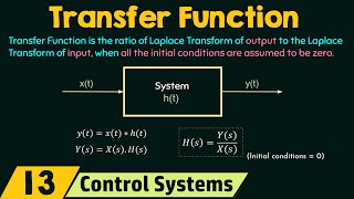
Transfer Function: Represents the ratio of output to input in Laplace domain, crucial for system analysis.
-
Laplace Transform: A technique used to analyze linear time-invariant systems in frequency domain.
-
Differential Equation: Governs the behavior of dynamic systems and forms the basis for deriving transfer functions.
Examples & Applications
Example of the mass-spring-damper system is used to derive the transfer function and analyze system behavior.
An instance where the transfer function is utilized for stability analysis in a control system design.
Memory Aids
Interactive tools to help you remember key concepts
Rhymes
To find the function that relates, factor and isolate the rates.
Stories
Imagine a spring that bounces in tune, mix forces and motion, and start to attune—a dancer in time, each twist a delight, the transfer function shows how it moves in the night.
Memory Tools
MFL: Model, Factor, Laplace for transfer functions.
Acronyms
G = 1 / (MS² + BS + K) helps remember the function structure.
Flash Cards
Glossary
- Transfer Function
A mathematical representation of the relationship between input and output in a dynamic system, expressed in the Laplace domain.
- Laplace Transform
A mathematical operation that transforms a time-domain function into a complex frequency domain representation.
- Differential Equation
An equation that describes the relationship between a function and its derivatives, often used in modeling dynamic systems.
Reference links
Supplementary resources to enhance your learning experience.