
Environmental Quality: Monitoring and Analysis
Enroll to start learning
You’ve not yet enrolled in this course. Please enroll for free to listen to audio lessons, classroom podcasts and take practice test.
Interactive Audio Lesson
Listen to a student-teacher conversation explaining the topic in a relatable way.
Introduction to Pollutant Transport Modeling
🔒 Unlock Audio Lesson
Sign up and enroll to listen to this audio lesson

Today we will explore how we model the transport of pollutants in the environment. Can anyone tell me what mass balance means in this context?

Is it about how much pollutant enters and leaves a certain area?
Exactly! The mass balance states that the rate of accumulation of pollutants equals the rate in minus the rate out. What happens if we assume there are no reactions in the area?

Then it simplifies the calculations since we only look at the flow in and out.
Correct! Recall this concept as the fundamental equation: Accumulation = Inflow - Outflow. It's vital when modeling concentrations.
Types of Dispersion Models
🔒 Unlock Audio Lesson
Sign up and enroll to listen to this audio lesson

In pollutant dispersion modeling, we have two main frameworks: Eulerian and Lagrangian models. Who can explain the difference?

The Eulerian model looks at fixed points in space, while the Lagrangian model follows the fluid flow.
Exactly! The Lagrangian model is especially useful for observing how pollutants move with the fluid. Remember, the Lagrangian perspective means we're focused on a 'puff' of pollution. Why is this significant?

Because it helps predict the behavior of pollutants at specific locations over time.
Right! This predictive capability is crucial for environmental monitoring.
Mathematical Models and Steady States
🔒 Unlock Audio Lesson
Sign up and enroll to listen to this audio lesson
Now, let’s look at the mathematical representation of dispersion in three dimensions. Can anyone summarize how we derive the concentration equation?
We look at a small volume of gas and apply the rate of inflow and outflow, assuming no reactions.
And we also include dispersion terms for each direction.
Precisely! We can then derive an equation that includes concentration changes over time. What’s the importance of steady states?
In a steady state, concentrations don’t change over time, indicating a constant inflow and outflow.
Correct! It’s crucial for simplifying our calculations and predicting environmental impacts.
Introduction & Overview
Read summaries of the section's main ideas at different levels of detail.
Quick Overview
Standard
This section provides an overview of how pollutants disperse in the environment, introducing the concepts of Eulerian and Lagrangian models, mass balance equations, and the significance of time and steady states in predicting concentrations of pollutants.
Detailed
Environmental Quality: Monitoring and Analysis
This section focuses on the critical task of modeling environmental pollutants through Gaussian dispersion models. Prof. Ravi Krishna from IIT Madras elucidates on how to predict the concentration of a pollutant, denoted as ρ A1, across different spatial dimensions (x, y, z) and over time. This involves understanding the principles of mass balance, which asserts that the rate of accumulation of a substance within a system is equal to the rate of inflow minus the rate of outflow, typically assuming no reactions occurring (for simplification).
Two primary models facilitate this dispersion modeling: Eulerian models, which are framed in fixed spatial positions, and Lagrangian models, which move with the fluid's flow. Prof. Krishna highlights that the Lagrangian model, where observations are made from the moving fluid's perspective, is more applicable here.
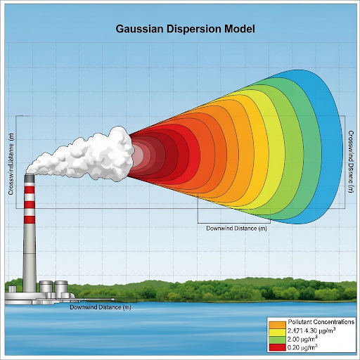
He discusses various factors affecting concentration—specifically, the emission rate from sources and how dispersion leads to the spread of pollutants over time and space. The section underscores the necessity of understanding steady states, which occur when concentrations do not change over time due to constant emissions and environmental stability. The mathematical representations of these concepts and their implications in real-world scenarios are also elaborated, making the section central to understanding environmental pollutant dynamics.
Youtube Videos


Audio Book
Dive deep into the subject with an immersive audiobook experience.
Introduction to Modeling Concentration
Chapter 1 of 4
🔒 Unlock Audio Chapter
Sign up and enroll to access the full audio experience
Chapter Content
So, our goal is to model the system to predict rho A1 as a function of x, y, z and time. This is our general prediction. If you are trying to invoke the mass balance and trying to develop mathematical models. Here two things may be happening: its rate in and rate out. The rate of accumulation equals rate in minus rate out plus there is no reaction (we are assuming no reactions here). This is an assumption because if you add reactions, then things will become very different. We are also considering only rho A1. This is just vapor phase concentration. We are not looking at particulate matter and all that. If you add that, then that is a different thing.
Detailed Explanation
In this section, we are trying to create a model to predict the concentration of a pollutant (rho A1). We look at how this concentration changes based on time and location (x, y, z). To predict this concentration, we focus on two main processes: how much pollutant enters a system (rate in) and how much leaves it (rate out). The accumulation is defined as the difference between these two rates. Importantly, we assume for simplicity that there are no chemical reactions altering the pollutant's concentration, although this assumption can be modified in more complex scenarios.
Examples & Analogies
Imagine you are filling a bathtub (the system) with water (pollutant). The rate at which you fill the tub (rate in) needs to be greater than the rate at which water is draining out (rate out) for the water level (concentration) to rise. If both rates are equal, the level stays the same, and if there is a leak (reaction), it complicates the situation. Here, we ignore the leak to simplify our understanding.
Types of Dispersion Models
Chapter 2 of 4
🔒 Unlock Audio Chapter
Sign up and enroll to access the full audio experience
Chapter Content
So dispersion models can be of two different kinds. One is called an Eulerian model, which is a fixed reference frame. What this means is, if I am modeling this room here. I am watching from here. So x equals 0 begins at that end and goes to this end. The Lagrangian model, on the other hand, is that you are moving with the fluid; the frame of reference is that body of fluid. So here dispersion model is set up as the most commonly used model. This is what is called the Lagrangian model.
Detailed Explanation
There are two main approaches to modeling how pollutants disperse in the environment: Eulerian and Lagrangian models. The Eulerian model observes changes at fixed points in space (like observing the room from one location), while the Lagrangian model tracks the movement of particles of fluid (like following a balloon in the wind). The Lagrangian model is often preferred for studying individual puffs or plumes of pollutants because it provides insights into how those pollutants move through the environment over time.
Examples & Analogies
Think of a traffic light. If you sit at the traffic light (Eulerian), you see how many cars pass every minute without moving with the cars. In contrast, if you are in a car and driving along with the other vehicles (Lagrangian), you experience traffic flow in a different way. You can gauge how quickly they move and how they interact with each other as you follow.
Understanding Plume Dynamics
Chapter 3 of 4
🔒 Unlock Audio Chapter
Sign up and enroll to access the full audio experience
Chapter Content
We are now looking at the plume (the entire system). When discussing the z and y axes and the dispersion, it references this particular system and not with reference to a fixed frame. The goal is to find out what will be the concentration at a particular distance x and at a particular height.
Detailed Explanation
In this part, the focus is on examining the plume of pollutants that is emitted into the atmosphere. As the plume rises and spreads, we observe the concentration of pollutants not in a static environment but relative to the movement of the plume itself. The goal is to understand how much pollutant concentration will be at various points in the plume, depending on its height (z) and distance (x) from its source. This dependency helps us determine exposure levels for individuals or the environment.
Examples & Analogies
Consider smoke rising from a chimney. The smoke (plume) spreads out as it moves up and disperses in the air. If you want to know how much smoke you would breathe in at a specific point downwind (at distance x and height), you need to consider how the smoke is rising and spreading in the wind, rather than just measuring from the ground.
Mathematical Representation of Dispersion
Chapter 4 of 4
🔒 Unlock Audio Chapter
Sign up and enroll to access the full audio experience
Chapter Content
So when we write the general equation, we have written down d rho A1/d t. Here I will change it to zero. I will derive this equation for you in a minute. We take a three-dimensional volume associated with the gas pollutants inside the plume. If there are no reactions here, the derivatives lead to an equation describing how the concentration changes over time and space.
Detailed Explanation
In this section, we start constructing the mathematical equations used to describe the dispersion of pollutants. By establishing a three-dimensional volume where the pollutants exist, we can analyze how concentration (rho A1) changes with time (d/Dt). Under our assumptions, we demonstrate that if there are no reactions influencing the concentration, we can simplify the representation into a more manageable mathematical form. This form allows us to model how pollutants disperse in the environment as a function of space and time.
Examples & Analogies
Imagine creating a map (the mathematical equation) of a river (the pollutant). The map helps you visualize how the water flows and what happens to it over specific areas and time periods. By knowing how the river behaves at different points (using our derived equations), you can predict where it might spread under various conditions.
Key Concepts
-
Pollutant Concentration Prediction: Understanding how to model and predict pollutant concentrations based on mass balance equations.
-
Dispersion Models: Differentiating between Eulerian and Lagrangian dispersion models for effective pollution analysis.
-
Steady State vs. Unsteady State: The implications of steady states in predicting environmental impacts.
Examples & Applications
An industrial facility releases a constant amount of a pollutant per hour into nearby air, demonstrating a steady state.
Using a Gaussian dispersion model to predict how a pollutant plume disperses in a residential area downwind from a factory.
Memory Aids
Interactive tools to help you remember key concepts
Rhymes
Pollutants flow, and then we know, mass balance keeps it in the flow.
Stories
Imagine a river where every drop enters just as another drop leaves—no drop stays behind. This represents steady state flow.
Memory Tools
Remember the acronym MEAL: Mass balance, Eulerian, Accumulation, Lagrangian to guide your understanding!
Acronyms
SPLAP for dispersion models
Steady State
Predictive behavior
Lagrangian model
Area measurement
Pollutants.
Flash Cards
Glossary
- Mass Balance
An equation stating that the rate of accumulation of a substance is equal to the rate of inflow minus the rate of outflow.
- Eulerian Model
A model that observes pollutants at fixed locations in space.
- Lagrangian Model
A model that follows the movement of pollutant plumes with the fluid flow.
- Steady State
A condition where the concentration of pollutants remains constant over time.
- Dispersion
The spreading of pollutants in the environment due to various factors over time.
Reference links
Supplementary resources to enhance your learning experience.