
Transport of Pollutants - Gaussian Dispersion Model
Enroll to start learning
You’ve not yet enrolled in this course. Please enroll for free to listen to audio lessons, classroom podcasts and take practice test.
Interactive Audio Lesson
Listen to a student-teacher conversation explaining the topic in a relatable way.
Introduction to Transport of Pollutants
🔒 Unlock Audio Lesson
Sign up and enroll to listen to this audio lesson

Today, we'll discuss how we model the transport of pollutants using the Gaussian dispersion model. Can anyone tell me what mass balance means in this context?

I think mass balance relates to how much pollutant we have coming in versus what is going out, right?
Exactly! The rate of accumulation equals the rate in minus the rate out, assuming no reactions are happening. This helps us track pollutants in various environments.

So, is this model practical for all kinds of pollutants?
Good question! This model primarily focuses on vapor phase concentrations and does not account for particulate matter unless adjustments are made.

What about the dispersion? How does that work?
Dispersion refers to the spreading of pollutants. This can occur in two main ways: Eulerian and Lagrangian models. We'll dive deeper into both.

Can you give us examples of how these models are applied in real life?
Most certainly! These models are used in environmental engineering to predict air quality and inform regulation strategies.
In summary, we've covered the basic idea of mass balance and how different models help us understand pollutant dispersion. Are there any questions?
Understanding Eulerian and Lagrangian Models
🔒 Unlock Audio Lesson
Sign up and enroll to listen to this audio lesson

Let's explore the key differences between the Eulerian model and the Lagrangian model for pollutant transport. Who can explain the Eulerian model?
The Eulerian model involves a fixed reference frame, meaning we measure pollutant concentrations at specific locations.
Correct! This model is useful when we want to understand the effect on a specific area over time. Now, how about the Lagrangian model?
The Lagrangian model tracks individual particles over time while they move through the plume. It follows their paths!
Exactly right! This model helps visualize how pollutants disperse from their source. Each model has its advantages depending on the situation.
In what scenarios would you use one model over the other?
Great question! The Eulerian model is often used for steady-state conditions, while the Lagrangian model is more beneficial for transient scenarios.
To summarize, the Eulerian model focuses on fixed positions while the Lagrangian model focuses on moving particles. This duality is critical for effective modeling.
Mathematical Formulation of Dispersion
🔒 Unlock Audio Lesson
Sign up and enroll to listen to this audio lesson
Now we’ll derive the equations from earlier discussions about dispersion. Can anyone recap the mass balance equation?
It's the rate of accumulation equals rate in minus rate out, right?
That's right! When we add terms to calculate dispersion, we also consider fluctuations in y and z, which can complicate our equations.
How do we simplify those equations for practical applications?
In many cases, we assume steady-state conditions, meaning concentrations don't change with time at a given location—that's very useful for prediction.
What about the role of environmental conditions in these equations?
Excellent point! We assume that wind speed and other conditions remain constant, which allows us to focus purely on pollutant transport.
To conclude, we've derived the dispersion equations and defined simplifying assumptions for modeling pollutant transport effectively.
Introduction & Overview
Read summaries of the section's main ideas at different levels of detail.
Quick Overview
Standard
This lecture focuses on modeling the transport of pollutants using the Gaussian dispersion model, emphasizing mass balance, different frames of reference (Eulerian and Lagrangian), and deriving equations for pollutant concentration over time. Key assumptions about reactions and steady-state conditions are also discussed.
Detailed
Detailed Summary
The Gaussian dispersion model is a widely used approach for predicting the concentration of pollutants in the atmosphere. It is based on the premise of mass balance, where the rate of accumulation of pollutants in a volume equals the rate of pollutants entering minus those leaving, disregarding any chemical reactions. This section introduces two essential frameworks for modeling dispersion: the Eulerian model, which utilizes a fixed reference frame to measure concentration at set points in space, and the Lagrangian model, which tracks individual fluid particles within the moving plume.
In this lecture, concentrations are examined primarily within the vapor phase, with insights on how pollutants disperse in atmospheric layers without considering particulate matter. The discussion progresses to derive the mathematical formulations necessary for describing this behavior, utilizing dimensions of space (x, y, z) and time. The significance of steady-state modeling is highlighted, underlining conditions where pollutant concentrations remain unchanged over time due to constant emission rates and environmental conditions. These concepts are crucial in pollution control and environmental engineering as they provide a foundation for predicting the impact of emission sources on air quality.
Youtube Videos


Audio Book
Dive deep into the subject with an immersive audiobook experience.
Modeling Pollution Transport
Chapter 1 of 5
🔒 Unlock Audio Chapter
Sign up and enroll to access the full audio experience
Chapter Content
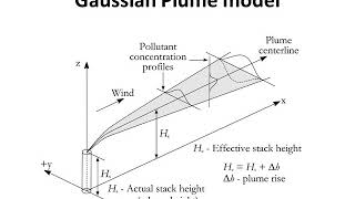
So, our goal is to model the system to predict rho A1 as a function of x, y, z and time, this is our general prediction. If you are trying to invoke the mass balance and trying to develop mathematical models. So, here two things may be happening, its rate in and rate out. So rate of accumulation equals rate in minus rate out plus there is no reaction (we are assuming no reactions here).
Detailed Explanation
In this part, we establish that our goal is to model the transport of pollutants, specifically how the concentration of a pollutant (denoted as rho A1) changes over time and space (x, y, z). The basic principle behind this is based on mass balance, which involves calculating the rate at which the pollutant enters and exits a given volume. The equation states that the change in pollutant concentration within that volume is equal to the amount coming in minus the amount going out, presuming no reactions occur (like degradation or chemical interactions). This simplifies our model, as we only focus on physical dispersion instead of chemical processes.
Examples & Analogies
Imagine a bathtub filling with water. The rate of water entering the bathtub can be thought of as the 'rate in,' while the rate of water draining out represents the 'rate out.' If the water is not spilling over the edge (no chemical reactions happening), the amount of water (the concentration of pollutants, in our case) filling up the tub can be predicted easily by measuring how fast it's filling and draining.
Types of Dispersion Models
Chapter 2 of 5
🔒 Unlock Audio Chapter
Sign up and enroll to access the full audio experience
Chapter Content
So dispersion models can be of two different kinds. One is called an Eulerian model, which is a fixed reference frame. What this means is, if I am modeling this room here. I am watching from here. Lagrangian model on the other hand is that you are moving with the fluid that is the frame of reference is that body of fluid.
Detailed Explanation
This section introduces two major types of dispersion models: Eulerian and Lagrangian. The Eulerian model observes changes from a fixed point in space, like watching the weather from a stationary station. In contrast, the Lagrangian model follows specific fluid particles as they move through space and time – akin to riding in a river and observing your surroundings as you float along. Each model has distinct applications and helps in visualizing and quantifying how pollutants disperse differently depending on the frame of reference.
Examples & Analogies
Picture watching a parade from the sidelines versus being part of the parade. In the Eulerian perspective (sidelines), you see the overall event unfold, while in the Lagrangian perspective (participating), you only see what's around you as you move along with the flow of the parade. Both perspectives provide valuable information, but focus on different elements of the same event.
Understanding Plume Behavior
Chapter 3 of 5
🔒 Unlock Audio Chapter
Sign up and enroll to access the full audio experience
Chapter Content
So here dispersion model is set up as the most commonly used model. This thing is what is called the Lagrangian model. We are now looking at the plume (we are looking at the entire system), but we are also seeing that when we are talking about the z and y and all that and the dispersion it is the reference to this particular, it is not with the reference to a fixed reference frame.
Detailed Explanation
The focus here is on how we manage and observe pollutant dispersion through the Lagrangian model by examining the behavior of a plume. The plume is essentially a cloud of pollutants released into the environment, and we’re more interested in how it spreads over time and in three dimensions rather than how a fixed location experiences its impact. This highlights the dynamic nature of dispersion, emphasizing the need to model both vertical and horizontal spreading in relation to the plume's movement.
Examples & Analogies
Think of a smoke signal rising from a campfire. Watching the smoke as it rises and spreads is similar to how the Lagrangian model views the plume of pollutants. If you’re walking with the smoke as it travels, you can observe how it curls and disperses over the landscape, giving you a better understanding of how air pollution behaviors change with environmental conditions.
Mathematical Representation of Dispersion
Chapter 4 of 5
🔒 Unlock Audio Chapter
Sign up and enroll to access the full audio experience
Chapter Content
So when we write the general equation, we have written down dA1. Here I will change it to zero. I will derive this equation for you in a minute. Let us say that we have a small volume. We take a three-dimensional volume. This is delta x, this is delta y, this is delta z.
Detailed Explanation
Here, we start delving into the mathematical formulation of the dispersion model. We use a three-dimensional volume represented by changes in the x, y, and z directions, denoted as delta x, delta y, and delta z. This allows us to systematically analyze how pollutants change within a prescribed volume, accounting for their movement and spreading due to turbulence and flow dynamics. It leads to the development of differential equations that describe the rate of change of pollutant concentration over time.
Examples & Analogies
Imagine measuring the extent of a puddle spreading outwards on a flat surface. You would look at small sections of the puddle ('delta x', 'delta y', 'delta z') to determine how quickly the water is moving into new areas. This local measurement can be related back to understand the whole layout of the puddle at larger scale, just as this approach helps us model the dispersion of pollutants in the environment.
Conditions for Unsteady State
Chapter 5 of 5
🔒 Unlock Audio Chapter
Sign up and enroll to access the full audio experience
Chapter Content
When will concentration change? Let us say if I have a plume here, so I am measuring concentration at this point. I would like to find out what is the concentration at this location which has a certain particular z, particular x, and some y. And at this point, if I want to measure concentration it will only be an unsteady state.
Detailed Explanation
In this part, we address the conditions under which we anticipate a change in the concentration of pollutants over time (unsteady state). If the concentration at a certain point remains constant over time, we refer to that as a steady state. However, if conditions like wind speed, source emissions of the pollutant, or environmental conditions vary, we will observe fluctuations in concentration. Understanding these conditions is crucial for predicting pollutant behavior accurately.
Examples & Analogies
Imagine standing by a riverbank and watching the water flow. If the river’s flow stays constant (same amount of water entering and exiting), changes at any point will be minimal, reflecting a steady state. However, if heavy rain suddenly causes more water to rush in, it alters the river’s flow downstream, illustrating how external changes can lead to an unsteady state and fluctuations in water levels.
Key Concepts
-
Mass Balance: The principle that the rate of accumulation equals the rate of inflow minus the rate of outflow.
-
Eulerian Model: A model that focuses on pollutant concentration at fixed spatial points.
-
Lagrangian Model: A model that tracks the movement of individual particles in a fluid medium.
-
Steady State Assumption: The condition where pollutant concentrations remain constant over time in a specific location.
Examples & Applications
Using the Gaussian dispersion model to predict the concentration of carbon monoxide emitted from a traffic intersection.
Applying the Eulerian model to assess pollutant levels in urban areas affected by industrial emissions.
Memory Aids
Interactive tools to help you remember key concepts
Rhymes
To keep pollutants in line, mass balance must be just fine; inflow, outflow, watch the time!
Stories
Imagine a river flowing steadily as pollutants are added. The balance of what comes in and what flows out keeps our river clean and safe.
Memory Tools
E-L-S (Eulerian-Lagrangian-Steady state) - Remember these three terms as the key concepts of pollutant transport.
Acronyms
G-D-M - Gaussian Dispersion Model stands for predicting air quality with flow patterns.
Flash Cards
Glossary
- Gaussian Dispersion Model
A mathematical model used to predict the concentration of pollutants in the atmosphere, based on assumed Gaussian distributions.
- Eulerian Model
A model of fluid flow that analyzes pollutant concentrations at fixed points in space.
- Lagrangian Model
A model that follows individual particles of fluid as they move through a flow field.
- Mass Balance
A principle stating that the rate of accumulation of a substance is equal to the rate of inflow minus the rate of outflow.
- Steady State
A condition where the concentrations of materials do not change over time at a given location, indicating constant inflows and outflows.
Reference links
Supplementary resources to enhance your learning experience.