
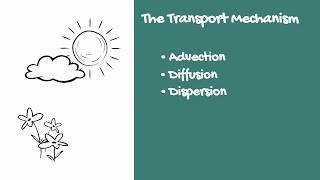
General Equation for Dispersion
Enroll to start learning
You’ve not yet enrolled in this course. Please enroll for free to listen to audio lessons, classroom podcasts and take practice test.
Interactive Audio Lesson
Listen to a student-teacher conversation explaining the topic in a relatable way.
Mass Balance in Dispersion Modeling
🔒 Unlock Audio Lesson
Sign up and enroll to listen to this audio lesson

Let's begin our discussion with the concept of mass balance in dispersion modeling. The basic idea is that the accumulation of a substance is equal to the rate of flow into the system minus the rate of flow out. Can anyone explain this idea further?

So, if we collect waste from an industrial plant, more waste entering than what we are treating would lead to accumulation, right?

And if the flow out equals the flow in, no accumulation occurs?
Exactly! This principle informs us about the dynamics of pollutant concentration in areas such as our environment. To help remember, think 'IN - OUT = ACCUMULATION'.
Do you remember the situation when there are reactions or degradation occurring? How might that affect accumulation?

I think reactions would mean that the input concentration might decrease even if we have constant flow in, right?
Great point! Reactions complicate our balance, signaling a need for further refinement in our modeling approach. Let's summarize: Mass balance is crucial for predicting concentration levels.
Dispersion Models: Eulerian vs. Lagrangian
🔒 Unlock Audio Lesson
Sign up and enroll to listen to this audio lesson

Moving forward, let’s distinguish between the two primary modeling frameworks: Eulerian and Lagrangian. Can anyone describe what an Eulerian model entails?
Isn't it based on a fixed point? Like observing pollution concentration in a specific location rather than following the pollutants?
Exactly, that’s the crux of Eulerian models. Now, how does a Lagrangian model differ?
It tracks the pollutants, moving along with them through the fluid, right?
Correct! Think of the Lagrangian model as riding along with the puff of smoke, observing how it spreads over time. Let’s use a mnemonic—'E for Eulerian, E for Fixed'; 'L for Lagrangian, L for Leading alongside.'

This makes more sense now! So, we often prefer Lagrangian for real-time dispersion modeling, especially in pollutant issue scenarios.
Absolutely! This distinction is crucial for our accurate applications in environmental quality assessments.
Deriving the General Dispersion Equation
🔒 Unlock Audio Lesson
Sign up and enroll to listen to this audio lesson
Now that we understand basic concepts, let's derive the general dispersion equation. What is the basic formula we need?
We start with the mass balance equation, right?
Yes! We then introduce terms for flow and dispersion in each direction. Can anyone guess what we incorporate for dispersion?
We apply Fick’s law which relates concentration gradients to diffusion flux?
Exactly! It’s the interplay between concentration gradients that shapes our dispersion behavior. As we step through the math, does everyone follow the terms as we integrate these components to form the equation?
It may look complex, but breaking it down with the individual flow contributions definitely helps!
Fantastic! Let’s summarize the main output—we have a representation for concentration change involving variables u, D, and spatial derivatives reflecting how pollutants move within the plume.
Steady-State vs Unsteady-State Conditions
🔒 Unlock Audio Lesson
Sign up and enroll to listen to this audio lesson
Shifting gears, let’s discuss when concentration might change during pollutant dispersion. What factors contribute to steady-state versus unsteady-state?
If conditions around the source remain constant, like constant emissions and wind speed, we see steady-state?
Exactly! In contrast, any fluctuation in output or environmental factors shifts us towards an unsteady state. Can anyone provide a practical scenario?
Like during a storm, if the wind speed changes, it could affect how pollutants disperse, causing unsteady conditions.
Right on target! In modeling scenarios, predicting unsteady-state may require more complex equations. Always think, 'constant conditions mean stable concentrations.'
It all comes together now! Understanding assumptions for our models is key.
Exactly! Each discussion item forms the building blocks we need for effective environmental monitoring.
Boundary Conditions in Dispersion Models
🔒 Unlock Audio Lesson
Sign up and enroll to listen to this audio lesson
Lastly, let’s focus on boundary conditions when solving our dispersion equations. Why are these conditions necessary?
They define how our system behaves at the limits! We need these for accurate modeling!
Correct! For instance, knowing concentration levels at the edges or physical boundaries helps us simplify our equations and find solutions. Any thoughts on types of boundary conditions?
We might have Dirichlet conditions, specifying certain values, and Neumann conditions related to gradients, right?
Perfect! Remember these types as they are crucial parameters in defining our model constraints!
I feel much more comfortable now with how boundary conditions impact our overall modeling!
Introduction & Overview
Read summaries of the section's main ideas at different levels of detail.
Quick Overview
Standard
Focusing on the mathematical modeling of pollutant transport, this section introduces the general equation for dispersion, differentiating between Eulerian and Lagrangian models. It elaborates on mass balance, the assumptions made during modeling, and the significance of steady-state conditions, providing insights into how concentration changes over time in various environmental contexts.
Detailed
In the section 'General Equation for Dispersion', we delve into the mathematical foundation of dispersion modeling in environmental studies, particularly concerning pollutant transport. The section begins by framing the goal of predicting concentration (B1A1) based on spatial coordinates (x, y, z) and time. Central to this modeling is the mass balance equation, which illustrates how accumulation equals the difference between rates of input and output, assuming no reactions take place. We explore two primary dispersion models: Eulerian, which utilizes a fixed reference frame, and Lagrangian, which follows the fluid’s path, with an emphasis on the more commonly applied Lagrangian perspective in plume modeling.
The derivation begins with a three-dimensional volume description involving specific dimensions and flow directions, highlighting dispersion in the context of pollutant dispersal. As the section progresses, it establishes a general equation for unsteady-state conditions using Fick’s law of diffusion, capturing the dynamic nature of concentration changes in relation to time. The importance of identifying factors such as source constancy and environmental conditions in modeling unsteady vs. steady states is also emphasized, laying the groundwork for practical applications in real-world environmental monitoring.
Youtube Videos


Audio Book
Dive deep into the subject with an immersive audiobook experience.
Understanding Dispersion Models
Chapter 1 of 4
🔒 Unlock Audio Chapter
Sign up and enroll to access the full audio experience
Chapter Content
So dispersion models can be of two different kinds. One is, what is called as an Eulerian model, which is a fixed reference frame. What this means is, if I am modeling this room here. I am watching from here. So x equals 0 begins at that end goes to this end start from here and here. Lagrangian model on the other hand is that you are moving with the fluid that is the frame of reference is that body of fluid.
Detailed Explanation
Dispersion models help us to understand how pollutants disperse in an environment. There are two main types of models: Eulerian and Lagrangian. The Eulerian model looks at specific locations in space, like a fixed point in a room, to study changes in pollutant concentration over time. Conversely, the Lagrangian model follows a specific fluid parcel and tracks how pollutants move with it. This is crucial for predicting the impact of pollutants at different points.
Examples & Analogies
Imagine you are watching cars in a traffic flow (Eulerian) versus being in one car and seeing where it goes (Lagrangian). In the former, you see how many cars pass a certain point over time, while in the latter, you experience the traffic from the driver's seat.
Modeling the Plume
Chapter 2 of 4
🔒 Unlock Audio Chapter
Sign up and enroll to access the full audio experience
Chapter Content
We are also seeing that when we are talking about the z and y and all that and the dispersion it is the reference to this particular, it is not with the reference to a fixed reference frame. This is the fixed reference frame where x equal to 0, the spreading itself is happening in each of these volumes. So, if you imagine one puff that is going out and this as a series of puffs that is coming out because there is rate at which this is emission is happening.
Detailed Explanation
When modeling the dispersion of pollutants, we observe their behavior in a larger context called a 'plume.' The plume consists of multiple 'puffs' of pollutant emissions that spread out as they move. The modeling focuses on how these puffs behave in terms of their spatial distribution, which is affected by the emissions' rate and environmental factors rather than a single reference point or location.
Examples & Analogies
Think of a smoke ring blown from your mouth. Each ring represents a 'puff' of smoke, and as it expands, it disperses into the air. The way the smoke spreads out is like how pollutants disperse in the environment, influenced by airflow and other factors.
General Equation Derivation
Chapter 3 of 4
🔒 Unlock Audio Chapter
Sign up and enroll to access the full audio experience
Chapter Content
So when we write the general equation, we have written it down. Let us say that we have a small volume. We take a three-dimensional volume. This is delta x, this is delta y, this is delta z. This is the volume inside one of the gas pollutants inside the plume.
Detailed Explanation
To derive the general equation for dispersion, we visualize a small three-dimensional volume within the pollutant plume, defined by small changes in the x, y, and z dimensions (delta x, delta y, delta z). This small volume allows us to analyze how the pollutant concentration (rho A1) changes within that space over time based on the concepts of mass flow (rate in, rate out) and dispersion.
Examples & Analogies
Imagine you are observing a small section of a river. If you know the flow rate of the water and the substances dissolving in it, you can predict how the concentration of those substances will change as you move downstream – this is similar to how we analyze small volumetric sections of air pollution.
Steady-State vs. Unsteady-State Analysis
Chapter 4 of 4
🔒 Unlock Audio Chapter
Sign up and enroll to access the full audio experience
Chapter Content
When will concentration change? Let us say if I have a plume here, so I am measuring concentration at this point. I would like to find out what is the concentration at this location which has a certain particular z, particular x and some y.
Detailed Explanation
In our analysis, we need to understand when the concentration of pollutants will change in a plume. This can be classified into 'steady-state' and 'unsteady-state' conditions. Steady-state means the concentration at a given point does not change over time; it remains constant. In contrast, unsteady-state means that environmental conditions, emissions, or other factors are leading to fluctuations in concentration.
Examples & Analogies
Consider a tap filling a bucket with water. If the tap flows steadily and the bucket has no leaks, the water level will rise steadily – that's steady-state. However, if you remove the tap suddenly or if water spills out, the level will fluctuate – that's unsteady-state.
Key Concepts
-
Mass Balance: The accumulation principle governing pollutant concentration changes.
-
Eulerian vs. Lagrangian Models: Distinctions between fixed point observations and tracking pollutants directly.
-
Fick’s Law: A foundational principle linking concentration gradients to diffusion flux in modeling pollution.
-
Steady-State vs. Unsteady-State Conditions: The impact of constant versus changing factors in pollutant concentration.
-
Boundary Conditions: Essential constraints for accurate solutions in mathematical models.
Examples & Applications
Accurate predictions of pollution dispersion in crowded urban areas where many factors influence pollutant spread.
Applying steady-state conditions to models assessing constant emissions from industrial sources.
Memory Aids
Interactive tools to help you remember key concepts
Rhymes
In flow or in puff, if you want to know rough, IN minus OUT, accumulation is tough!
Stories
Imagine a river carrying debris. If nothing changes in the inflow and outflow, the debris concentration stays constant!
Memory Tools
E for Eulerian (E for Earth) measures at fixed points. L for Lagrangian (L for Letting flow) tracks along with the motion.
Acronyms
M.A.C (Mass balance, Accumulation, Consistency) to remember the core principles of mass balance in concentrations.
Flash Cards
Glossary
- Mass Balance
The principle that states accumulation in a system is equal to the rate of input minus the rate of output.
- Eulerian Model
A fixed reference frame model used to analyze pollution concentration over time at specific points in space.
- Lagrangian Model
A model that follows the path of pollutants as they move through their environment.
- Fick’s Law
A principle describing diffusion that states the flux of a substance is proportional to its concentration gradient.
- SteadyState Conditions
Conditions where the concentration at a specific location does not change over time.
- UnsteadyState Conditions
Conditions where concentration at a specific location changes over time due to varying factors.
- Boundary Conditions
Constraints applied to the mathematical model to define how it behaves at the limits of the domain.
Reference links
Supplementary resources to enhance your learning experience.