
Next Steps: Gaussian Dispersion Model Derivation
Enroll to start learning
You’ve not yet enrolled in this course. Please enroll for free to listen to audio lessons, classroom podcasts and take practice test.
Interactive Audio Lesson
Listen to a student-teacher conversation explaining the topic in a relatable way.
Introduction to Pollution Models
🔒 Unlock Audio Lesson
Sign up and enroll to listen to this audio lesson

Welcome everyone! Today we're going to discuss pollution models, focusing on the Gaussian dispersion model. Can someone tell me what a dispersion model is?

Isn't it a way to predict how pollutants spread in the environment?
Exactly! Dispersion models help us foresee concentrations of pollutants based on various factors. We mainly talk about two types: Eulerian and Lagrangian models.

What's the difference between those two?
Good question! In an Eulerian model, we are looking from a fixed point, like a room, whereas in a Lagrangian model, we follow the fluid particles themselves, moving with the flow.

So does that mean Lagrangian models are more dynamic?
Yes, exactly, they can represent how the plume evolves over time. Let's keep these concepts in mind as we move forward!
Mass Balance Approach
🔒 Unlock Audio Lesson
Sign up and enroll to listen to this audio lesson

Now, let’s delve into the mass balance approach. Can anyone explain what mass balance entails?
I think it’s about how mass enters and leaves a system?
Absolutely! The general equation states that the rate of accumulation equals the rate of input minus the rate of output. Here, we assume no reactions are occurring.

If we add reactions, how will it change the equation?
Great point! Adding reactions complicates the model because we would have to account for different rates of transformation and degradation of pollutants.
So we're focusing only on one pollutant?
Correct! We're focusing on `rho A1`, the concentration of a specific pollutant.
Advection & Dispersion Formulations
🔒 Unlock Audio Lesson
Sign up and enroll to listen to this audio lesson
Let's now look at the equations derived from our mass balance. We use Fick's law for dispersion, which illustrates how pollutants disperse through the flowing medium.
What does the term dispersion mean in this context?
Good question! Dispersion refers to the spreading of pollutant particles from areas of high concentration to low concentration.
And how do we incorporate both advection and dispersion in the equation?
Excellent inquiry! The equation combines terms for advection, which is the movement due to upstream velocity and diffusion that accounts for uneven dispersal.
Can you remind us how steady state affects our model?
Absolutely! Under steady-state conditions, concentrations don't change over time, allowing us to simplify our calculations.
Boundary Conditions
🔒 Unlock Audio Lesson
Sign up and enroll to listen to this audio lesson
Finally, let’s talk about boundary conditions. Why do you think they are crucial when solving these equations?
I guess they help define the limits of our area of study?
Exactly! They provide essential constraints that dictate how pollutants might behave within specific dimensions.
Can you give an example of boundary conditions?
Sure! For instance, conditions could specify that pollution concentration is zero at a certain distance from a source.
So we need to include three conditions based on x, y, and z?
Exactly right! This accounts for the three-dimensional space we're working within.
Introduction & Overview
Read summaries of the section's main ideas at different levels of detail.
Quick Overview
Standard
In this section, the derivation of the Gaussian dispersion model is explored, highlighting the assumptions made in the mathematical modeling of pollutant transport, particularly regarding the mass balance and the distinction between Eulerian and Lagrangian models.
Detailed
The Gaussian dispersion model is crucial for predicting the concentration of pollutants over time and space. This section begins with establishing a mass balance approach, considering the rate of accumulation of pollutants without reactions, leading to the development of a mathematical representation for pollutant transport. It distinguishes between Eulerian models, where the focus is on fixed points in space, and Lagrangian models, which track moving fluid particles. By analyzing dispersion within a plume, the section breaks down the governing equations, incorporating terms for advection and dispersion according to Fick’s law. The importance of steady-state assumptions and boundary conditions in solving the derived equations is emphasized, setting the stage for further exploration of Gaussian dispersion methodologies.
Youtube Videos


Audio Book
Dive deep into the subject with an immersive audiobook experience.
Introduction to Dispersion Models
Chapter 1 of 5
🔒 Unlock Audio Chapter
Sign up and enroll to access the full audio experience
Chapter Content
So dispersion models can be of two different kinds. One is, what is called as an Eulerian model, which is a fixed reference frame. What this means is, if I am modeling this room here. I am watching from here. So x equals 0 begins at that end goes to this end start from here and here. Lagrangian model on the other hand is that you are moving with the fluid that is the reference frame is that body of fluid.
Detailed Explanation
Dispersion models are crucial for studying how pollutants disperse in the environment. There are two main types of dispersion models: Eulerian and Lagrangian. The Eulerian model treats the environment as a fixed point, where the observer remains stationary, and the concentration of pollutants is observed as they move through different locations over time. In contrast, the Lagrangian model tracks the particles as they move with the fluid, treating them as points in time and space. This difference is essential for understanding how pollutants behave in different scenarios, especially when considering the influence of wind and other environmental factors.
Examples & Analogies
Think of the Eulerian model like observing traffic flow through a fixed camera set up at an intersection. You see cars coming and going but don’t move with them. On the other hand, the Lagrangian model is akin to riding in a car and observing the road and environment change as you drive. Both perspectives give useful information about traffic, but the data you gather will vary depending on whether you remain stationary or move with the cars.
Understanding the Puff Concept
Chapter 2 of 5
🔒 Unlock Audio Chapter
Sign up and enroll to access the full audio experience
Chapter Content
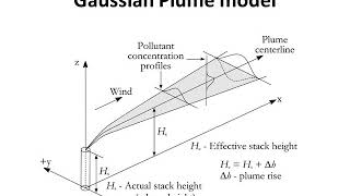
So here dispersion model is set up as the most commonly used model. This thing is what is called the Lagrangian model. We are now looking at the plume (we are looking at the entire system), but we are also seeing that when we are talking about the z and y and all that and the dispersion it is the reference to this particular, it is not with the reference to a fixed reference frame.
Detailed Explanation
In this context, the term 'puff' refers to a discrete volume of pollutants released into the air. The Lagrangian model allows us to focus on this puff and understand how it dissipates and spreads with wind and other factors. The key point is that the dispersion does not regard a fixed observer; we look at the pollutant as it moves and its distance from the source. This perspective is crucial when predicting concentrations at various points in the environment based on the puff's behavior.
Examples & Analogies
Imagine blowing a bubble with bubblegum. As the bubble expands, it changes shape and size, influenced by air currents. The Lagrangian model is like tracking the bubble's growth and movement through the air while it's floating, rather than just standing still and observing its location intermittently. This helps us understand where the bubble might float in the future and how it will interact with its surroundings.
Dispersion Terms in the Equation
Chapter 3 of 5
🔒 Unlock Audio Chapter
Sign up and enroll to access the full audio experience
Chapter Content
Sowhenwewritethegeneralequation,wehavewrittenindowndC,hereIwillchangeittozero. Nowletussaythatwehaveasmallvolume. Wetakeathree-dimensionalvolume. Thisisdeltax,thisisdelta y,thisisdeltaz.
Detailed Explanation
Here we begin to build our mathematical representation of how the dispersion works in three dimensions. We look at small volumes defined by delta x, delta y, and delta z. These dimensions allow us to analyze how pollutants enter and leave a specific volume, providing insights into the accumulation and distribution of concentrations. Flow rates in these directions help us derive foundational equations that explain how pollutants disperse in various scenarios.
Examples & Analogies
Think of a small block of cheese placed in a corner of a large room filled with air. If the cheese starts to release a smell (the pollutant), we can analyze it by dividing the air in the room into small cubes (the small volume). Each cube can then be observed for how much of the smell it contains, how it enters and leaves, and which direction it spreads. This way, we can predict how soon someone will smell the cheese depending on where they are in the room.
Flux and Dispersion Equation
Chapter 4 of 5
🔒 Unlock Audio Chapter
Sign up and enroll to access the full audio experience
Chapter Content
Sothex-directionfluxislikethisandtheareaitgoesthroughthiswhichisdeltaxdelta y deltaz pluswehaveanothertermwhichisy-n dispersion,y+deltaywhichisinthisdirection.
Detailed Explanation
The flux of pollutants refers to how much of the substance passes through a unit area over a certain time. In our equations, we incorporate various dispersion terms that characterize how pollutants spread in the x, y, and z directions. By examining these fluxes, we can elucidate the contributions from each directional spread, leading to a more comprehensive understanding of how pollutants behave in three-dimensional space.
Examples & Analogies
Imagine a sprinkler watering a garden. The amount of water passing through a specific section of the garden is akin to flux, influenced by how far the water travels in different directions. If one part of the garden gets soaked while another remains dry, we can analyze the 'dispersion' pattern to understand where most water is and adjust the sprinkler’s angle to ensure an equal distribution in all areas.
General Equation and Assumptions
Chapter 5 of 5
🔒 Unlock Audio Chapter
Sign up and enroll to access the full audio experience
Chapter Content
Now so you can write this equation like this daurhoA1dautequalsDxdausquarerhoA1bydau x square + Dy dau y square + Dz - u of x.
Detailed Explanation
We conclude by outlining the general equation that represents the behavior of the pollutants over time and space. This combined equation integrates the effects of various dispersion coefficients and the flow velocity. The assumptions made here suggest that factors such as constant emission rates and steady environmental conditions are in play, which simplifies our modeling and solutions, making it practical for real-world applications.
Examples & Analogies
Consider a river flowing steadily while factories release pollutants into it at a consistent rate. If we assume the river's flow speed and water quality remain constant, we can predict how far and how quickly the pollutants spread through the river. This predictability is crucial for regulators and environmental scientists to understand potential impacts on aquatic life downstream.
Key Concepts
-
Mass Balance Approach: Summarizes inputs and outputs of pollutants in the system, providing foundational equations for modeling.
-
Advection vs. Dispersion: Highlights the distinction between the movement of pollutants with fluid flow (advection) and their spread due to concentration gradients (dispersion).
-
Eulerian vs. Lagrangian Models: Differentiates between fixed reference points and following fluid paths over time, crucial for understanding pollutant transport.
-
Steady State vs. Unsteady State: Explores the assumptions needed to simplify equations for practical applications.
Examples & Applications
An industrial plant releasing a constant pollutant flow allows for steady-state assumptions in Gaussian modeling.
In urban planning, understanding how pollutants disperse from traffic systems involves applying Lagrangian models for accurate predictions.
Memory Aids
Interactive tools to help you remember key concepts
Rhymes
Pollutants flow with the breeze, spreading wide as you please.
Stories
Imagine a balloon releasing air in a still field, where the air represents pollutants drifting in silence, showcasing how they spread over time.
Memory Tools
Remember 'EASE' for Eulerian's fixed points and 'LAW' for Lagrangian following fluid paths.
Acronyms
M.A.D for Mass Balance, Advection, Dispersion – the key to understanding pollution models.
Flash Cards
Glossary
- Dispersion Model
A mathematical representation predicting the spread of pollutants in the environment.
- Eulerian Model
A fixed reference frame tracking stationary points in space.
- Lagrangian Model
A model that follows moving fluid elements through space and time.
- Mass Balance
An equation that represents the input, output, and accumulation of mass in a system.
- Advection
The transport of substances by the bulk motion of fluid.
- Dispersion
The process of pollutants spreading in the environment due to various factors.
- Steady State
A condition where the concentration of pollutants remains constant over time.
- Boundary Condition
Constraints applied to variables at the boundary of the solution domain.
Reference links
Supplementary resources to enhance your learning experience.