
Fourier Integrals
Enroll to start learning
You’ve not yet enrolled in this course. Please enroll for free to listen to audio lessons, classroom podcasts and take practice test.
Interactive Audio Lesson
Listen to a student-teacher conversation explaining the topic in a relatable way.
Introduction to Fourier Integrals
🔒 Unlock Audio Lesson
Sign up and enroll to listen to this audio lesson

Today, we are diving into Fourier Integrals. Unlike Fourier Series, which work with periodic functions, Fourier Integrals handle non-periodic functions. Can anyone think of an example of a non-periodic function?

How about a temperature distribution in a long rod?
Exactly! Temperature in a rod can vary continuously and isn’t repetitive. This is where Fourier Integrals come in.

So, is it correct that Fourier Integrals represent a continuous superposition of sines and cosines?
Correct! This allows us to effectively analyze non-periodic functions. Remember, we can think of this as continuously layering waves.

Are there specific applications for this in engineering?
Great question! Applications include solving heat conduction problems and vibrations in structures. Let’s summarize: Fourier Integrals are a bridge to handle non-periodic functions effectively in engineering applications.
Derivation and Integral Form
🔒 Unlock Audio Lesson
Sign up and enroll to listen to this audio lesson

Now moving on to the derivation of the Fourier Integral from Fourier Series. Starting with the series for a finite interval, what happens as we let L approach infinity?

I believe the sum transitions into an integral form!
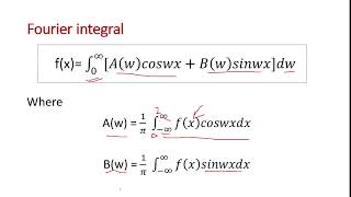
Exactly! The discrete coefficients become continuous. The formula is: \( f(x) = \int_{0}^{\infty} [A(\omega)\cos(\omega x) + B(\omega)\sin(\omega x)] d\omega \). Who can explain why we need both $A(\omega)$ and $B(\omega)$?
They represent how much of each sine and cosine function is needed to recreate the original function!
Correct! This integral preserves the functionality of Fourier Series but for non-periodic contexts. Summarizing, we can express a variety of functions continuously through this integral.
Applications in Engineering
🔒 Unlock Audio Lesson
Sign up and enroll to listen to this audio lesson
Let’s discuss some real-world applications of Fourier Integrals in civil engineering. Can someone name a scenario where these might be useful?
Heat conduction in a long concrete beam sounds like a good example!
Absolutely! When there’s an instantaneous point heat source, Fourier Integrals help predict how heat spreads through the structure. Can anyone think of another application?
What about analyzing vibrations in a bridge?
Yes! The vibration analysis of continuous structures makes use of Fourier Integrals to understand how structures react to non-periodic loadings. To summarize, Fourier Integrals are invaluable for accurately modeling complex physical phenomena.
Example Problems and Solutions
🔒 Unlock Audio Lesson
Sign up and enroll to listen to this audio lesson
Now let’s solve some problems using Fourier Sine and Cosine integrals. First, who can evaluate the Fourier sine integral for this function?
We start by identifying that the function is odd, so we use only sine integrals.
Exactly! And what do we find for $B(\omega)$?
It involves integrating $f(t)sin(\omega t) dt$. We can look for known integrals for $e^{−ax}$ too!
Great teamwork! These integrals facilitate our understanding of how to explicitly apply Fourier methods. Leaning on example problems allows us to sharpen our skills in applying the concepts we learned.
Understanding Conditions for Fourier Integrability
🔒 Unlock Audio Lesson
Sign up and enroll to listen to this audio lesson
Let’s clarify the conditions required for a function to have a valid Fourier Integral. Who can list one?
The function needs to be piecewise continuous, right?
Exactly! And what about absolute integrability?
It should be absolutely integrable over the entire range.
Perfect! Thus, any discontinuities must be finite in magnitude. Summarizing, to use Fourier Integrals, a function must meet these strict criteria.
Introduction & Overview
Read summaries of the section's main ideas at different levels of detail.
Quick Overview
Standard
In this section, we explore the necessity and application of Fourier Integrals in representing non-periodic functions. We derive the Fourier Integral formula from Fourier Series and discuss its significance, particularly in Civil Engineering, where it aids in solving problems related to heat conduction, vibration analysis, and dynamic analysis of structures.
Detailed
Fourier Integrals
Introduction
Fourier Integrals are introduced to represent non-periodic functions, which cannot be adequately captured by Fourier Series. In many engineering applications, such as heat conduction and vibrations, non-periodic phenomena are common, necessitating the use of Fourier Integrals.
Derivation and Formula
The Fourier Integral formula derives from the transition of discrete Fourier coefficients in Fourier Series to a continuous representation, resulting in:
$$ f(x) = \int_{0}^{\infty} [A(\omega)\cos(\omega x) + B(\omega)\sin(\omega x)] d\omega $$
where $A(\omega)$ and $B(\omega)$ are coefficients representing the function. The complex Fourier integral form is also discussed, simplifying the representation.
Properties and Applications
Conditions for Fourier Integrability are outlined, emphasizing the importance of piecewise continuous and absolutely integrable functions. The section highlights engineering applications, including:
- Heat conduction in semi-infinite rods
- Vibration analysis of structures
- Dynamic loading scenarios in soil mechanics
Examples and Worked Problems
Examples illustrate how to compute Fourier sine and cosine integrals, providing practical insights into their application in engineering contexts.
In summary, Fourier Integrals are essential tools for engineers, facilitating the analysis and solution of complex problems involving non-periodic functions.
Youtube Videos


Audio Book
Dive deep into the subject with an immersive audiobook experience.
Introduction to Fourier Integrals
Chapter 1 of 16
🔒 Unlock Audio Chapter
Sign up and enroll to access the full audio experience
Chapter Content
In practical applications, especially in Civil Engineering, many physical phenomena such as heat conduction, vibrations in structures, and signal transmission are best described using functions that may not be periodic. While Fourier Series is a powerful tool for representing periodic functions, it becomes inadequate when dealing with non-periodic functions. To handle such cases, Fourier Integrals are introduced. A Fourier Integral allows us to express a non-periodic function as a continuous superposition of sines and cosines (or exponential functions), making it indispensable in solving engineering problems involving non-periodic boundary conditions and transient phenomena.
Detailed Explanation
The introduction to Fourier Integrals highlights their importance in contexts where the data and functions we deal with are not periodic - meaning they don't repeat over regular intervals. For example, processes like heat diffusion or vibrations in engineering structures occur continuously and do not return to a starting point in a predictable manner. This is where Fourier Integrals come into play, as they extend the Fourier Series concept, allowing us to work with a continuous set of sine and cosine functions to capture the full behavior of non-periodic phenomena.
Examples & Analogies
Think about how you hear various sounds. The sounds produced by a musical instrument (like a piano) are periodic; they have a repeating pattern. On the other hand, the noise from a busy street is not periodic and varies continuously. Just like how you would need different techniques to analyze the music versus the street noise, engineers use Fourier Integrals to analyze continuous heat flow or vibrations in buildings.
The Need for Fourier Integrals
Chapter 2 of 16
🔒 Unlock Audio Chapter
Sign up and enroll to access the full audio experience
Chapter Content
Fourier Series represents a function f(x) defined on a finite interval [−L,L] as an infinite sum of sines and cosines:
∞
f(x)=a_0 + ∑(a_n cos(nπx/L) + b_n sin(nπx/L))
But for non-periodic functions or when the interval becomes infinitely large (L→∞), the discrete nature of the Fourier coefficients becomes continuous, and the sum becomes an integral. This transition leads us to Fourier Integrals.
Detailed Explanation
Here, we learn that the traditional Fourier Series works well for functions defined over a specific range, usually a finite interval. However, when we deal with functions that extend over an infinite area or do not repeat at all, the series cannot effectively convey their properties. Hence, the concept shifts from discrete sums (as in Fourier Series) to continuous integrals, which allows for capturing the behavior of functions across an unbounded space using Fourier Integrals.
Examples & Analogies
Imagine trying to measure the continuous flow of a river. If you only took periodic measurements at specific points, you'd miss the fluctuations happening in between those measurements. However, if you had a continuous flow gauge that could track every single change, you would get a complete picture. Similar to this, Fourier Integrals provide a way to analyze all the details of a continuous function without missing critical information.
Derivation of the Fourier Integral
Chapter 3 of 16
🔒 Unlock Audio Chapter
Sign up and enroll to access the full audio experience
Chapter Content
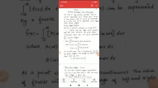
Let f(x) be a piecewise continuous function on (−∞,∞) that satisfies the Dirichlet conditions and is absolutely integrable, i.e.,
∫(−∞ to ∞) |f(x)|dx < ∞. We begin with the Fourier series of f(x) defined on [−L,L]:
f(x)= ∑(a_n cos(nπx/L) + b_n sin(nπx/L))
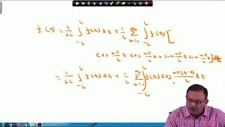
Let ω = nπ. As L → ∞, ω → ω becomes a continuous variable. The sum becomes an integral:
f(x)= ∫(0 to ∞) [A(ω)cos(ωx) + B(ω)sin(ωx)] dω
Where,
A(ω)= (1/π) ∫(−∞ to ∞) f(t)cos(ωt)dt, B(ω)=(1/π)∫(−∞ to ∞) f(t)sin(ωt)dt. This is the Fourier Integral Representation of f(x).
Detailed Explanation
This chunk explains how we develop the formula for a Fourier Integral. We start again with a function that meets certain conditions (piecewise continuous and integrable). By taking the Fourier series, we note that as the interval L increases indefinitely, the coefficients related to the sine and cosine functions seamlessly transition from a discrete to a continuous framework, leading us to integrate over all possible frequencies. The new function described through A(ω) and B(ω) represents the input function across every point versus just specific intervals.
Examples & Analogies
Imagine assembling a huge puzzle (the continuous function) where each piece represents a tiny frequency making up that picture. Each piece is like a sine or cosine wave. Traditional Fourier series would allow you to put together only a limited number of pieces at a time. However, by switching to Fourier Integrals, you can lay down all the pieces continuously on the table, allowing for a complete assembly of the whole picture, capturing all nuances of the function.
Fourier Integral Formula
Chapter 4 of 16
🔒 Unlock Audio Chapter
Sign up and enroll to access the full audio experience
Chapter Content
Let f(x) be a function such that:
• f(x) is piecewise continuous on (−∞,∞)
• f(x) is absolutely integrable over (−∞,∞)
Then,
f(x)= ∫(0 to ∞) [A(ω)cos(ωx) + B(ω)sin(ωx)] dω,
Where:
A(ω)= (1/π) ∫(−∞ to ∞) f(t)cos(ωt)dt, B(ω)=(1/π)∫(−∞ to ∞) f(t)sin(ωt)dt.
Alternatively, combining cosine and sine terms, we can express the function using the complex Fourier integral:
f(x)= (1/(2π)) ∫(−∞ to ∞) fb(ω)e^(iωx)dω,
Where:
fb(ω)= ∫(−∞ to ∞) f(t)e^(-iωt)dt. This is the Fourier Transform of f(x).
Detailed Explanation
This segment introduces the formalized formula which represents a function using Fourier Integrals. We summarize what conditions f(x) must meet for a valid formulation and derive two forms: one using sine and cosine, another using complex exponentials. The complex form simplifies the representation, allowing for easier manipulation in mathematical operations, particularly in engineering applications.
Examples & Analogies
Think of translating a song into a different language. The traditional Fourier integral methods (sine/cosine terms) represent a direct translation, while the complex Fourier form can be thought of as using older dialects or simpler forms that capture the emotion and style of the original, no matter the language used. This represents how engineers can efficiently analyze signals without losing the original information.
Fourier Cosine and Sine Integrals
Chapter 5 of 16
🔒 Unlock Audio Chapter
Sign up and enroll to access the full audio experience
Chapter Content
If f(x) is even (i.e., f(−x)=f(x)), then its Fourier integral contains only cosine terms:
f(x)= ∫(0 to ∞) A(ω)cos(ωx)dω.
If f(x) is odd (i.e., f(−x)=−f(x)), then its Fourier integral contains only sine terms:
f(x)= ∫(0 to ∞) B(ω)sin(ωx)dω.
This simplification is useful in boundary value problems involving symmetric domains.
Detailed Explanation
Here, the characteristics of the function's symmetry greatly influence its Fourier integral representation. Even functions lead to cosine representations, while odd functions convert to sine representations. This distinction simplifies the calculations and understanding of boundary value problems in physics and engineering, particularly in structures where symmetry plays a role.
Examples & Analogies
Consider a seesaw on a playground. When two kids of equal weight sit at both ends, it balances perfectly - this is like an even function. If they both sit on one side, it tips, reflecting an odd function. Engineers can analyze these types of structures more easily when they can identify symmetry, thus applying the appropriate Fourier integral form based on the situation.
Conditions for Fourier Integrability
Chapter 6 of 16
🔒 Unlock Audio Chapter
Sign up and enroll to access the full audio experience
Chapter Content
For a function f(x) to possess a valid Fourier Integral representation:
1. f(x) must be piecewise continuous in every finite interval of R.
2. f(x) must be absolutely integrable over (−∞,∞).
3. Discontinuities must be finite and of finite magnitude.
If these conditions are satisfied, then:
lim (f(x+ϵ) + f(x−ϵ)) = 2f(x)
ϵ→0
at all points of continuity.
Detailed Explanation
This section outlines the necessary conditions to ensure that a function can be correctly represented by a Fourier Integral. The function must be continuous within any segment and integrable over the entire real line. Additionally, if there are any points where the function jumps or behaves oddly, these should be limited in number and extent. A crucial property discussed is the behavior at points of continuity, indicating that as we approach a point, the values should converge to double the function's value at that point.
Examples & Analogies
Think of a bridge – it needs to be stable at every point to safely support weight. If we apply this idea to functions, the requirements for Fourier integrability are like ensuring that the bridge's foundation is secure, with no weak points (discontinuities). If these conditions are met, the structure (function) will adequately support the load (analysis) required without collapse or miscalculation.
Applications in Civil Engineering
Chapter 7 of 16
🔒 Unlock Audio Chapter
Sign up and enroll to access the full audio experience
Chapter Content
Fourier Integrals are particularly important in Civil Engineering for solving:
• Heat conduction problems in infinite or semi-infinite rods
• Vibration analysis of continuous beams or plates
• Dynamic analysis of structures subject to non-periodic loading
• Soil mechanics for propagation of stress waves
• Ground motion analysis during earthquakes
For example, temperature distribution in a long concrete beam due to an instantaneous point source can be solved using the Fourier integral method.
Detailed Explanation
This section presents the significant role that Fourier Integrals play in practical engineering applications. They are essential in areas such as analyzing how heat spreads within materials or understanding vibrations in structures. By employing Fourier Integrals, engineers can model complex real-world behaviors, making them crucial tools in design and evaluation under conditions that don't fit traditional, periodic models.
Examples & Analogies
Imagine putting a hot pack on one end of a long piece of metal. Over time, the heat travels along the metal – this is akin to Fourier Integrals modeling the process. Engineers need to understand how quickly and effectively that heat will transfer if they’re designing a component that needs to remain cool under stress, such as in engines or hot machinery.
Worked Examples
Chapter 8 of 16
🔒 Unlock Audio Chapter
Sign up and enroll to access the full audio experience
Chapter Content
Example 1:
Evaluate the Fourier sine integral representation of the function:
f(x) = {
1, 0<x<a
0, x≥a
}
Solution:
Since f(x) is odd over (0,∞), use the sine integral:
f(x)= ∫(0 to ∞) B(ω)sin(ωx) dω.
Where:
B(ω)= (1/π) ∫(0 to a) sin(ωt) dt = (1−cos(ωa))/(πω).
Thus,
f(x)= ∫(0 to ∞) (1−cos(ωa))sin(ωx) dω/πω.
Example 2:
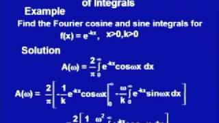
Find the Fourier cosine integral of f(x)=e^(-ax), a>0, for x>0.
Use:
f(x)= ∫(0 to ∞) A(ω)cos(ωx) dω.
Where:
A(ω)= (1/(π)) ∫(0 to ∞) e^(-at)cos(ωt) dt = 2a/(a^2 + ω^2).
Thus,
f(x)= ∫(0 to ∞) (2a/(a^2 + ω^2))cos(ωx)/π dω.
Detailed Explanation
In this section, we see two worked examples illustrating how to compute Fourier sine and cosine integrals. The first example involves a piecewise function, breaking it down into usable sine forms for easy calculations. The second example provides a representation of an exponential decay function as a Fourier cosine integral. This illustrates how practical applications often call for integrating over the frequency spectrum, revealing the function's characteristics.
Examples & Analogies
Think of a chef following a recipe where each ingredient equates to sections of a function. For the sine and cosine integrals, you are combining and measuring different ingredients (the sine and cosine waves) to produce a final dish (the overall function). Each step in the worked example is akin to carefully adding each ingredient, ensuring the final meal comes together perfectly.
Dirichlet’s Integral
Chapter 9 of 16
🔒 Unlock Audio Chapter
Sign up and enroll to access the full audio experience
Chapter Content
A useful result in Fourier Integrals is:
∫(0 to ∞) (sin(ωx)/ω) dω = {π/2, x>0; 0, x=0; −π, x<0}.
This integral frequently appears in solving boundary value problems using Fourier methods.
Detailed Explanation
This result is known as Dirichlet's Integral and serves as an important reference point in many Fourier-related calculations. It reveals how oscillating functions like sine relate to their frequency components and provides useful boundaries when solving physical problems in various domains.
Examples & Analogies
Imagine you are releasing a pebble in different depths of water. The ripples create waves that spread differently, and depending on where you are (above or below the water), it affects how you perceive them. Similarly, Dirichlet's Integral connects various behaviors of sine functions across different scenarios and reveals vital links in problem-solving, particularly in engineering.
Complex Form of Fourier Integral
Chapter 10 of 16
🔒 Unlock Audio Chapter
Sign up and enroll to access the full audio experience
Chapter Content
So far, we have discussed the Fourier integral in terms of sine and cosine functions. However, it is often more convenient and elegant to express it using complex exponentials. Let f(x) be an absolutely integrable function over (−∞,∞). Then the complex Fourier integral representation of f(x) is:
f(x)= (1/(2π)) ∫(−∞ to ∞) fb(ω)e^(iωx) dω,
Where the Fourier transform fb(ω) is defined as:
fb(ω)= ∫(−∞ to ∞) f(t)e^(-iωt) dt.
The inverse Fourier transform is:
f(x)= (1/(2π)) ∫(−∞ to ∞) fb(ω)e^(iωx) dω.
Detailed Explanation
This segment introduces the complex form of the Fourier Integral, using exponentials instead of sines and cosines. This form not only unifies the representation, making it more flexible but also simplifies solving differential equations and integrating various mathematical techniques in engineering practices. By employing complex numbers, computations become less cumbersome and increasingly versatile.
Examples & Analogies
Using a GPS system is like using the complex form. While you can track your location with multiple directions (sine and cosine), the GPS simplifies everything down to straight, calculated coordinates (complex exponentials), making navigation so much easier and efficient. Thus, the complex form streamlines complex processes similarly to how GPS navigates routes.
Properties of the Fourier Transform
Chapter 11 of 16
🔒 Unlock Audio Chapter
Sign up and enroll to access the full audio experience
Chapter Content
Understanding the properties of the Fourier Transform helps in efficiently solving various problems. Let f(x) ↔ fb(ω) denote the Fourier transform pair.
- Linearity:
F[af(x) + bg(x)] = a fb(ω) + b g b(ω). - Translation (Shift):
• In the time domain:
F[f(x−a)] = e^(−iωa) fb(ω).
• In the frequency domain:
F[e^(iaxf(x))] = fb(ω−a). - Scaling:
F[f(ax)] = (1/|a|) fb(ω/a). - Differentiation:
If f(x) is differentiable,
F[(df(x)/dx^n)] = (iω)^n fb(ω).
This is particularly useful for solving PDEs.
Detailed Explanation
In this section, we dissect the Fourier Transform's key properties which allow for systematic manipulation of functions across various contexts. The linearity property illustrates that a combination of inputs yields a proportionate output in the transformed domain. Translation, scaling, and differentiation provide tools for adjusting functions with respect to shifts in space or frequency which are important when working with differential equations.
Examples & Analogies
Consider tuning a radio. You can adjust the dial (translation) to switch between channels, change the volume (scaling), or shift the tone (differentiation). Just as these adjustments allow you to find the right sound, the properties of Fourier Transform give engineers and scientists the flexibility to manipulate and analyze signals effectively in various applications.
Fourier Integral in Engineering Problem Solving
Chapter 12 of 16
🔒 Unlock Audio Chapter
Sign up and enroll to access the full audio experience
Chapter Content
Let’s look at how the Fourier Integral is applied in a real engineering scenario.
Problem: Heat Diffusion in a Semi-Infinite Rod.
A rod of infinite length initially at zero temperature receives an instantaneous unit heat source at x=0 at t=0. The governing equation is the one-dimensional heat equation:
∂u/∂t = α² ∂²u/∂x²
With initial condition:
u(x,0) = δ(x)
And boundary condition:
u(±∞,t) = 0
Taking the Fourier Transform in x, we convert the PDE to an ODE:
∂u(ω,t)/∂t = −α²ω²u(ω,t).
Solving gives:
u(ω,t) = e^(−α²ω²t).
Taking the inverse Fourier transform:
u(x,t) = (1/(2π)) ∫(−∞ to ∞) e^(−α²ω²t)e^(iωx) dω.
Using the standard Gaussian integral identity:
u(x,t) = (1/√(4πα²t)) e^(−(x²/4α²t)).
This is the heat kernel, a fundamental solution showing how heat diffuses through the rod — a crucial result for civil engineers analyzing thermal effects in structures.
Detailed Explanation
This chunk explains a practical engineering example using Fourier Integrals related to heat diffusion in a semi-infinite rod. The heat equation describes how heat spreads over time, and by applying the Fourier Transform, we can convert complex partial differential equations into simpler algebraic ones that are easier to solve. The final result showcases a standard form known as the heat kernel, which engineers use to predict temperature distributions in various scenarios.
Examples & Analogies
If you've ever put your hand on a radiator, you experience heat diffusion firsthand. The way heat spreads throughout the radiator resembles the mathematical modeling of heat flow described in this section. Engineers use the principles of Fourier Integrals similarly to predict how heat will affect structures and materials over time after an instantaneous heat event.
Parseval’s Theorem for Fourier Integrals
Chapter 13 of 16
🔒 Unlock Audio Chapter
Sign up and enroll to access the full audio experience
Chapter Content
Parseval's identity relates the energy of a signal in time domain to that in frequency domain. Let f(x) and g(x) be absolutely integrable functions. Then:
∫(−∞ to ∞) f(x)g(x) dx = (1/(2π)) ∫(−∞ to ∞) fb(ω)g b(ω) dω.
When f = g, it becomes:
∫(−∞ to ∞) |f(x)|² dx = (1/(2π)) ∫(−∞ to ∞)|fb(ω)|² dω.
This has practical importance in energy calculations, error estimation, and signal processing in structural monitoring systems.
Detailed Explanation
In this section, we introduce Parseval's Theorem, which offers a relationship between the total energy of a signal viewed in both time and frequency domains. This theorem is beneficial for engineers as it allows them to analyze how energy is conserved and shifts between these two perspectives. It ensures that energy represented by a function remains equivalent, whether viewed as a signal in time or its frequency representation.
Examples & Analogies
Consider a painter who uses different colors (the various frequencies of a signal) but blends them to create a single shade (the time domain signal). No matter how the colors are mixed, in the end, they should have a proportion reflecting the total amount of paint used. Similarly, Parseval’s theorem assures that regardless of how a function’s components are mixed, the total energy remains consistent and accurately reflected across its representations.
Comparison: Fourier Series vs Fourier Integral
Chapter 14 of 16
🔒 Unlock Audio Chapter
Sign up and enroll to access the full audio experience
Chapter Content
Feature Fourier Series Fourier Integral
Applicable to Periodic functions Non-periodic functions
Domain Finite interval Infinite interval
Representation Discrete sum of Continuous integral
sines/cosines
Coefficients a_n,b_n A(ω),B(ω) or fb(ω)
Use in Engineering Vibrations of bounded Heat transfer, infinite
structures domain analysis.
Detailed Explanation
This comparison highlights the primary differences between Fourier Series and Fourier Integrals. While Fourier Series are ideal for periodic functions defined over a limited domain, Fourier Integrals extend that analysis to non-periodic functions across infinite domains. The key takeaway is that each method serves specific cases based on the nature of the function.
Examples & Analogies
Think about a pendulum swinging (periodic function) where you can predict its motion with a Fourier Series versus the waves in the ocean (non-periodic function) that change constantly. Fourier Series captures the pendulum's regularity, while Fourier Integrals analyze the complex, ever-changing nature of ocean waves.
Common Integral Forms for Reference
Chapter 15 of 16
🔒 Unlock Audio Chapter
Sign up and enroll to access the full audio experience
Chapter Content
To aid problem-solving, here are standard Fourier integral forms:
1. Fourier Sine Transform of f(x)=1, 0
Detailed Explanation
This segment provides common forms of Fourier transforms that are frequently needed for practical applications. These forms help expedite computations in signal processing and engineering problems. They serve as handy references for quickly solving related integrals without deriving every time.
Examples & Analogies
Imagine having a toolbox where each essential tool is at your fingertips for quick fixes (the standard integral forms). When something breaks, rather than creating a new tool every time, you reach for the one already designed for the job. Similarly, these common Fourier integral forms are pre-built solutions ready for immediate application in engineering calculations.
Exercises
Chapter 16 of 16
🔒 Unlock Audio Chapter
Sign up and enroll to access the full audio experience
Chapter Content
- Derive the Fourier cosine integral of f(x)=xe^(-x) for x>0.
- Evaluate the Fourier sine integral of the step function:
f(x)={
1, 0<xL
} - Use the complex Fourier integral to represent f(x)= 1/(1+x²).
- Apply Fourier integral methods to solve the initial value problem for the one-dimensional wave equation.
- Show that the function f(x)=e^(-a|x|) has a Fourier transform and compute it.
Detailed Explanation
This section presents exercises designed to reinforce the concepts covered in the chapter. Each problem guides students through deriving and applying Fourier integrals to various functions and scenarios, promoting active learning and practical application of theory.
Examples & Analogies
These exercises act like workout challenges in a gym—each task is designed to help you build your strength (knowledge) bit by bit. Just as athletes need to train on different skills (weightlifting, cardio), students need to tackle diverse problems to become proficient in applying Fourier Integrals and understanding their use in engineering.
Key Concepts
-
Fourier Integrals: Tool for representing non-periodic functions using sines and cosines.
-
Dirichlet Conditions: Essential criteria for the existence of Fourier Integrals.
-
Applications in Engineering: Includes heat conduction, vibration analysis, and dynamic loads.
Examples & Applications
Examples illustrate how to compute Fourier sine and cosine integrals, providing practical insights into their application in engineering contexts.
In summary, Fourier Integrals are essential tools for engineers, facilitating the analysis and solution of complex problems involving non-periodic functions.
Memory Aids
Interactive tools to help you remember key concepts
Rhymes
Fourier's ways of sine and cosine, help us make non-periodic lines.
Stories
Imagine a bridge vibrating under a non-periodic load; Fourier Integrals allow engineers to model its response accurately.
Memory Tools
Remember 'P.A.F' for conditions: Piecewise continuous, Absolutely integrable, Finite discontinuities.
Acronyms
DCAF
Dirichlet Conditions for Fourier Expansions
Flash Cards
Glossary
- Fourier Integral
A mathematical representation of a non-periodic function as a continuous sum of sine and cosine functions.
- Integrability
A property indicating whether a function can be integrated over a specific range.
- Dirichlet Conditions
A set of conditions that a function must satisfy to ensure the existence of its Fourier series or integral.
- Piecewise Continuous
A function that is continuous on each piece of its domain except at a finite number of points.
- Absolutely Integrable
A function whose absolute value can be integrated over the entire real line.
Reference links
Supplementary resources to enhance your learning experience.