
Two-Port Network Interconnections
Interactive Audio Lesson
Listen to a student-teacher conversation explaining the topic in a relatable way.
Introduction to Two-Port Network Interconnections
🔒 Unlock Audio Lesson
Sign up and enroll to listen to this audio lesson

Good morning, everyone! Today, we're diving into the world of two-port networks interconnections. To start, can anyone explain what a two-port network actually is?

Is it a circuit with two pairs of terminals where you can connect inputs and outputs?
Exactly! And when we combine multiple two-port networks, we create more complex systems while still keeping their individual characteristics. Can someone tell me some applications of this?

Cascaded amplifiers and filters, right?
Correct! Those are key applications. Remember, we can use two-port networks for impedance matching as well.
In short, these networks allow us to analyze and design more sophisticated electrical systems.
Series and Parallel Connections
🔒 Unlock Audio Lesson
Sign up and enroll to listen to this audio lesson

Now let's explore the fundamental methods of interconnection. First, we have the series connection. Who can describe how the Z-parameters behave in this case?

I believe the Z-parameters add together, right?
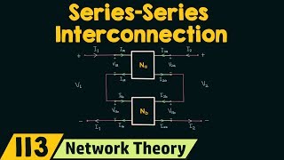
Perfect! The combined Z-matrix is expressed as Z_total = Z_A + Z_B. Remember, both input and output currents must be equal, I₁ = I₁' and I₂ = I₂'.

What about parallel connections?
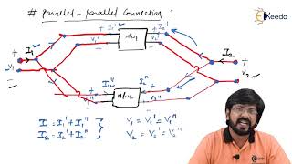
Good question! In parallel connections, Y-parameters are added, and we need the input voltages to be identical. So what’s the combined formula here?
Y_total = Y_A + Y_B!
Absolutely right! Understanding both methods is essential for circuit design and analysis.
Cascade Connections and Stability
🔒 Unlock Audio Lesson
Sign up and enroll to listen to this audio lesson
Next up is the cascade connection, a vital technique in amplifier design. Can someone explain how we combine the ABCD matrices in this case?
We multiply them together, right? ABCD_total = ABCD_A × ABCD_B!
Yes! This method is prevalent in amplifiers and filters. Now, what other factors should we consider when designing these stages?
Loading effects and stability,
Great! The stability of our networks is crucial, and we can use the Rollett Stability Factor. It needs to be greater than one for stability. Can anyone summarize what we learnt about stability today?
K > 1 and we watch for the Δ parameter condition?
Exactly! This ensures that our circuits remain stable during operation.
Applications and Practical Examples
🔒 Unlock Audio Lesson
Sign up and enroll to listen to this audio lesson
Finally, let’s talk about some practical design examples. Who can describe a basic application of cascaded amplifiers?
In a CE-CC configuration, we can make higher total gains by multiplying the individual stage gains!
Exactly! And what’s the total gain formula?
A_V(total) = A_V1 × A_V2!
Right on! And in filter design, how do we set up a ladder filter?
By connecting series inductors and shunt capacitors to form a bandpass filter!
You've all grasped the concepts beautifully! Two-port networks are fundamental in designing efficient electronic systems.
Introduction & Overview
Read summaries of the section's main ideas at different levels of detail.
Quick Overview
Standard
The section delves into various methods for interconnecting two-port networks—namely series, parallel, and cascade connections. It discusses how these interconnections maintain individual network characteristics and highlights their applications, such as in amplifier design and impedance matching. Practical considerations like loading effects and stability analysis are also addressed.
Detailed
Two-Port Network Interconnections
In this section, we examine the interconnection methods of two-port networks, which involve combining multiple such networks to create more complex systems while preserving their individual characteristics. The primary interconnection methods are series, parallel, and cascade configurations.
Key Interconnection Methods
- Series Connection: In this method, the Z-parameters of the networks add together. For series connections, input and output currents must remain equal. The resulting Z-matrix is expressed as:
\[ Z_{total} = Z_A + Z_B \]
- Parallel Connection: This involves adding Y-parameters together under the condition that input/output voltages must be identical. The total Y-matrix is:
\[ Y_{total} = Y_A + Y_B \]
- Cascade Connection: The most common method for amplifiers and filters, where the ABCD matrices of the systems multiply together:
\[ ABCD_{total} = ABCD_A \times ABCD_B \]
Advanced Topologies
The section also outlines advanced interconnection topologies, such as series-parallel and parallel-series combinations. Each method uses its respective parameter set (h-parameters and g-parameters) and involves similar addition concepts.
Practical Considerations
Real-world applications must consider loading effects and stability trends, utilizing metrics like the Rollett Stability Factor (K) to assess network behavior.
Applications
Practical applications of these techniques are seen in cascaded amplifier design and ladder filter configurations, showcasing their relevance in electronic design.
In summary, understanding two-port network interconnections is crucial for designing efficient electrical systems, making this knowledge foundational for engineers.
Youtube Videos


Audio Book
Dive deep into the subject with an immersive audiobook experience.
Introduction to Network Interconnections
Chapter 1 of 10
🔒 Unlock Audio Chapter
Sign up and enroll to access the full audio experience
Chapter Content
8.1 Introduction to Network Interconnections
- Definition:
- Combining multiple two-port networks to form more complex systems while preserving their individual characteristics
- Key Applications:
- Cascaded amplifier stages
- Filter design (low-pass, high-pass, bandpass)
- Impedance matching networks
Detailed Explanation
This section introduces the concept of two-port network interconnections, where we combine multiple two-port networks into a more complex system. The goal is to maintain the unique characteristics of each network while enabling them to work together effectively. Some of the primary applications of this technique include creating cascaded amplifier stages, designing filters such as low-pass, high-pass, or bandpass filters, and developing impedance matching networks that ensure optimal power transfer between circuits.
Examples & Analogies
Think of two-port network interconnections like a music band where each musician represents a two-port network. Each musician has their own unique sound, and when they play together, they create a new, harmonious piece of music. Just like in a band, each individual musician retains their characteristics, while together they form a complete song.
Fundamental Interconnection Methods
Chapter 2 of 10
🔒 Unlock Audio Chapter
Sign up and enroll to access the full audio experience
Chapter Content
8.2 Fundamental Interconnection Methods
8.2.1 Series Connection (Z-Parameters Add)
Network A Network B
Z1 Z2
V1─┬─□□□──┬──□□□─┬─V2
│ │ │
I1 I1' I2
- Combined Z-Matrix:
\[Z_{total} = Z_A + Z_B\] - Conditions:
- Input currents must be equal (I₁ = I₁')
- Output currents must be equal (I₂ = I₂')
8.2.2 Parallel Connection (Y-Parameters Add)
+──Network A──+
│ │
V1─┤ ├─V2
│ │
+──Network B──+
- Combined Y-Matrix:
\[Y_{total} = Y_A + Y_B\] - Conditions:
- Input voltages must be identical
- Output voltages must be identical
8.2.3 Cascade Connection (ABCD Matrices Multiply)
V1─Network A─┬─Network B─V2
│
I1'=I2'
- Combined ABCD Matrix:
\[ABCD_{total} = ABCD_A × ABCD_B\] - Most common for amplifier stages and filter design
Detailed Explanation
This section covers three fundamental methods for interconnecting two-port networks: series, parallel, and cascade connections. In a series connection, the Z-parameters of the networks add up, requiring that the input and output currents are equal. In a parallel connection, Y-parameters are combined, which requires that the input and output voltages are equal. The cascade connection is where ABCD matrices multiply together, and it is particularly common in amplifier stages and filter designs where we need to analyze how successive stages interact with each other.
Examples & Analogies
Consider a series connection like water flowing through pipes connected end-to-end. Each pipe has a characteristic resistance to flow, and the total resistance is the sum of each pipe’s resistance. In a parallel connection, imagine multiple pipes that are side by side, all delivering water to a bucket. The total capacity is the sum of water from all pipes, provided the pressure remains the same across all inlets.
Advanced Interconnection Topologies
Chapter 3 of 10
🔒 Unlock Audio Chapter
Sign up and enroll to access the full audio experience
Chapter Content
8.3 Advanced Interconnection Topologies
8.3.1 Series-Parallel (h-Parameters Add)
Network A
│
├─Network B
│
- Combined h-Matrix:
\[h_{total} = h_A + h_B\]
8.3.2 Parallel-Series (g-Parameters Add)
Network A
│
┼─Network B
│
- Combined g-Matrix:
\[g_{total} = g_A + g_B\]
Detailed Explanation
In this section, we explore two advanced interconnection topologies: series-parallel and parallel-series connections. The series-parallel connection combines the h-parameters of the networks, allowing additional flexibility in designing transistor circuits. The parallel-series connection involves combining g-parameters, which is often used in feedback networks. These advanced interconnection techniques allow for greater complexity and functionality in circuit design, tailoring connections to specific requirements of electronic applications.
Examples & Analogies
Think of series-parallel connections like a power strip in a home where some devices are plugged in end-to-end (series) while others are plugged into different outlets (parallel). This configuration allows different devices to be powered simultaneously, accommodating varying power needs just like these interconnection methods adapt to circuit design requirements.
Practical Considerations
Chapter 4 of 10
🔒 Unlock Audio Chapter
Sign up and enroll to access the full audio experience
Chapter Content
8.4 Practical Considerations
8.4.1 Loading Effects
- Impedance Mismatch:
\[
ext{Actual gain} = rac{A_V}{1 + Z_{out}/Z_{in}}
\] - Solution: Use buffer stages (emitter/source followers)
8.4.2 Stability Analysis
- Rollett Stability Factor (K):
\[
K = rac{1 - |S_{11}|^2 - |S_{22}|^2 + | ext{Δ}|^2}{2|S_{12}S_{21}|}
\]
where \(Δ = S_{11}S_{22} - S_{12}S_{21}\)
Detailed Explanation
This section highlights the practical considerations when designing two-port networks, focusing on loading effects and stability analysis. Impedance mismatch can significantly alter the expected gain of a network, and the loading effects must be considered to ensure accurate measurement and functionality. One common solution to impedance issues is using buffer stages, which prevent loading effects from adversely affecting a circuit’s performance. Additionally, the stability of active networks can be determined using the Rollett Stability Factor (K), which provides conditions under which the network operates reliably without oscillation or instability.
Examples & Analogies
Imagine a water hose connected to a sprinkler. If the hose has too big or too small of a nozzle (impedance mismatch), the sprinkler won’t work efficiently. Similarly, just as you might add a water pressure booster (buffer stage) to improve flow, stabilizing a network ensures that it functions properly and efficiently without causing any overflow or unwanted spraying.
Design Examples
Chapter 5 of 10
🔒 Unlock Audio Chapter
Sign up and enroll to access the full audio experience
Chapter Content
8.5 Design Examples
8.5.1 Cascaded Amplifier Design
Stage 1 (CE) Stage 2 (CC)
Z1 Z2
V1─□□□─┬─────────□□□─V2
│ ▲
└─Coupling Cap
- Total Gain:
\[A_{V(total)} = A_{V1} × A_{V2}\]
8.5.2 Ladder Filter Design
Series L Shunt C Series L
V1─□□□─┬───||───┬───□□□─V2
│ │
GND GND
- ABCD Matrix Multiplication:
\[ABCD_{filter} = ABCD_L × ABCD_C × ABCD_L\]
Detailed Explanation
In this section, we examine practical design examples of cascading amplifiers and designing ladder filters. In cascaded amplifier design, the total voltage gain is the product of the individual gains from each stage, making it crucial to understand how each stage impacts overall performance. The ladder filter design demonstrates how various components (inductors and capacitors) are arranged to achieve the desired frequency response using ABCD matrix multiplication, allowing engineers to craft filters that meet specific signal processing needs.
Examples & Analogies
Designing cascaded amplifiers can be thought of as building a multi-story building where each floor (amplifier stage) adds to the total height (gain). Each floor must be designed to support the next, just like each amplifier stage must function well to ensure the total gain is optimal. On the other hand, a ladder filter can be likened to a series of steps (inductors and capacitors) that guide water down to a desired level, filtering out unwanted debris, similar to how a filter passes only certain frequencies while blocking others.
Verification Methods
Chapter 6 of 10
🔒 Unlock Audio Chapter
Sign up and enroll to access the full audio experience
Chapter Content
8.6 Verification Methods
8.6.1 Experimental Verification
- Impedance Measurements:
- Network Analyzer for S-parameters
- LCR meter for Z/Y parameters
- Signal Tracing:
- Input test signal, measure output at each stage
8.6.2 Simulation Techniques
* Cascaded Amplifier Example
X1 1 2 CE_Amplifier
X2 2 3 CC_Buffer
.subckt CE_Amplifier ...
.subckt CC_Buffer ...
.ac dec 10 1Hz 100MHz
.probe V(3)/V(1)
.end
Detailed Explanation
This section discusses methods for verifying the designs of two-port networks, emphasizing the importance of both experimental and simulation techniques. Experimental verification can involve measuring impedances using a network analyzer or LCR meter, as well as signal tracing to test actual performance across stages. Simulation techniques using circuit design software allow engineers to test their designs virtually, which is essential for validating performance before physical implementation. This dual approach ensures that designs behave as expected under various conditions.
Examples & Analogies
Consider this like building a model before constructing a house. Engineers create a scaled version of their design using software simulations to envision how it will perform. Once the model is satisfactory, they build the real structure, much like verifying circuit designs through real measurements before finalizing them in the physical world.
Summary Table: Interconnection Methods
Chapter 7 of 10
🔒 Unlock Audio Chapter
Sign up and enroll to access the full audio experience
Chapter Content
8.7 Summary Table: Interconnection Methods
| Connection | Parameter Used | Combination Rule | Application |
|---|---|---|---|
| Series | Z-parameters | Matrix addition | High-Z circuits |
| Parallel | Y-parameters | Matrix addition | Low-Z circuits |
| Cascade | ABCD-parameters | Matrix multiplication | Amplifier chains |
| Series-Parallel | h-parameters | Matrix addition | Transistor models |
| Parallel-Series | g-parameters | Matrix addition | Feedback networks |
Detailed Explanation
Here we have a summary table that concisely outlines different interconnection methods used in two-port networks. Each method specifies the type of parameters involved (Z, Y, ABCD, h, g), the rule for combining them (either through addition or multiplication), and typical applications for each type of connection. Understanding this table provides a quick reference for choosing the appropriate interconnection strategy based on the circuit requirements.
Examples & Analogies
This table is similar to a menu at a restaurant listing different dishes (interconnection methods) available, the ingredients (parameters) used in those dishes, and the preparation style (combination rules). Just as you would choose a dish based on your taste (application), engineers select network configurations that best suit their specific needs.
Key Equations
Chapter 8 of 10
🔒 Unlock Audio Chapter
Sign up and enroll to access the full audio experience
Chapter Content
8.8 Key Equations
- Cascaded Networks:
\[
\begin{bmatrix}
V_1 \
I_1
\end{bmatrix}
=
\begin{bmatrix}
A_1 & B_1 \
C_1 & D_1
\end{bmatrix}
\begin{bmatrix}
A_2 & B_2 \
C_2 & D_2
\end{bmatrix}
\begin{bmatrix}
V_2 \
-I_2
\end{bmatrix}
\] - Stability Criterion:
\[
K > 1 ext{ and } | ext{Δ}| < 1
\]
Detailed Explanation
This section presents key equations relevant to two-port networks. The first equation indicates how to represent cascaded networks using a matrix form, showing how voltages and currents interact across different networks. The second equation provides the stability criterion for a network, specifying the conditions under which a network will remain stable without oscillation. These equations are critical for analyzing and designing reliable electronic systems.
Examples & Analogies
Think of these equations like recipes that outline the steps and ingredients needed to create a dish (circuit design). The first equation details how to combine multiple flavors (circuit behaviors) into a final meal (total response), while the stability criterion serves as a quality check to ensure every dish tastes good and doesn’t spoil (maintain stability in circuit operations).
Laboratory Experiment
Chapter 9 of 10
🔒 Unlock Audio Chapter
Sign up and enroll to access the full audio experience
Chapter Content
8.9 Laboratory Experiment
8.9.1 Cascaded RC Networks
- Setup:
- Stage 1: R=1kΩ, C=100nF (low-pass)
- Stage 2: R=1kΩ, C=10nF (high-pass)
- Measurements:
- Individual and combined frequency response
- Compare measured vs. calculated ABCD parameters
- Expected Results:
- Bandpass characteristic (f_L ≈ 160Hz, f_H ≈ 16kHz)
- -6dB/octave roll-off on both sides
Detailed Explanation
This section outlines a practical laboratory experiment focusing on cascaded RC (resistor-capacitor) networks. The setup involves two stages with specific resistor and capacitor values to create a low-pass and high-pass filter. The experiment includes taking frequency response measurements to observe how the combination of these stages produces a bandpass characteristic. This hands-on approach helps students understand theoretical concepts practically by comparing actual results with theoretical predictions.
Examples & Analogies
Conducting this laboratory experiment can be likened to tuning a musical instrument. Just as musicians adjust strings and air flow to achieve the desired sound qualities (results), students adjust resistors and capacitors in their circuits to produce specific filters, revealing how theoretical designs translate into practical outcomes.
Summary
Chapter 10 of 10
🔒 Unlock Audio Chapter
Sign up and enroll to access the full audio experience
Chapter Content
8.10 Summary
- Interconnection method determines which parameter set to use
- Cascade connections are most common in signal processing
- Loading effects must be accounted for in practical designs
- Stability is critical for active networks
Detailed Explanation
In the final section, we summarize the key points discussed throughout the chapter. The choice of interconnection method is crucial as it influences the parameters used for analysis and design. Cascade connections are highlighted as prevalent in signal processing applications, underscoring their importance. It's also emphasized that loading effects must be taken into account to ensure accurate performance, and finally, stability is deemed essential for the reliable operation of active networks.
Examples & Analogies
Summarizing the section is like distilling a long movie into its main plot points. Just as viewers need to grasp the essential elements of a narrative to understand its significance, engineers must focus on the key aspects of interconnections, such as methods, applications, and considerations, to effectively design and analyze electronic circuits.
Key Concepts
-
Two-Port Network: A fundamental circuit concept for analyzing circuits with two pairs of terminals.
-
Z-Parameters: Used in series connections to define the voltage and current relationship.
-
Y-Parameters: Relevant for parallel connections, illustrating current-voltage relationships.
-
ABCD Matrices: Essential in cascading networks for calculating overall performance.
-
Loading Effects: Important to consider to avoid instability and performance loss in network design.
Examples & Applications
In a series connection of two resistive networks, Z_total is simply the sum of their impedances.
For parallel connected capacitors, Y_total is the sum of their admittances, allowing for parallel operations in filtering applications.
Memory Aids
Interactive tools to help you remember key concepts
Rhymes
In series the currents stay the same, together they form a harmonious game.
Stories
Imagine a city connected by roads (the networks). Each road allows cars (currents) to travel. In series, every car must stop at each crossroad (each network), while in parallel, cars can take different roads, but all must depart from the same intersection (equal voltages).
Memory Tools
S-PAC: Series connections, Parallel current, Amplification Cascade. Remember this to recall the connection types.
Acronyms
ABCDE
ABCD for cascading
for buffers
for combined parameters
for design.
Flash Cards
Glossary
- TwoPort Network
An electrical network with two pairs of terminals for input and output connections.
- ZParameters
Parameters that define the relationship between voltage and current in a two-port network, specifically in series connections.
- YParameters
Parameters used to describe the relationship of currents and voltages in a network, specifically applicable in parallel configurations.
- ABCD Matrices
A set of parameters defined for two-port networks that describe input-output relationships in cascaded networks.
- Loading Effects
Effects that arise when connecting additional circuits to a network, potentially affecting the network's performance due to impedance mismatch.
- Stability Analysis
The study of a system to ensure that it maintains stable behavior under varying input conditions.
Reference links
Supplementary resources to enhance your learning experience.