
Discrete-Time Signal Representation
Interactive Audio Lesson
Listen to a student-teacher conversation explaining the topic in a relatable way.
Introduction to Discrete-Time Signals
🔒 Unlock Audio Lesson
Sign up and enroll to listen to this audio lesson

Today, we're going to explore how we represent continuous-time signals as discrete-time signals. Can someone tell me what a discrete-time signal actually is?

Isn't it just when we take samples of a continuous signal at specific intervals?
Exactly! A discrete-time signal is produced by sampling a continuous signal, like x(t), at regular intervals. This is mathematically represented as x[n] = x(nT). What can you tell me about 'T' in this equation?

T is the sampling period, right? It's the time interval between each sample!
Great! And how do we relate the sampling period to sampling frequency?

Oh, is it fs = 1/T? So, if we increase the sampling rate, the sampling period decreases!
Correct! This understanding is foundational for both sampling and signal processing as a whole.
Mathematical Representation of Discrete-Time Signals
🔒 Unlock Audio Lesson
Sign up and enroll to listen to this audio lesson

Now, let’s explore how we mathematically represent a continuous-time signal through sampling. Can anyone remind me of the notation used for discrete-time signals?

We use x[n] for discrete-time signals and x(t) for continuous signals, right?
Absolutely! So, if we choose a continuous signal x(t), sampling it produces the sequence x[n]. For example, if we sample every 1 ms, we would use T = 0.001 seconds. What does that make the sampling frequency?
That would be 1,000 Hz, since fs = 1/T!
Exactly! And this is crucial since the choice of fs impacts our ability to accurately reconstruct the continuous signal from its samples.
Importance of Sampling in Signal Processing
🔒 Unlock Audio Lesson
Sign up and enroll to listen to this audio lesson
Let’s discuss why sampling is important. What can happen if we don't sample at a high enough frequency?
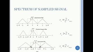
We could end up with aliasing, where high-frequency components get misinterpreted as lower frequencies!
Correct! That's known as aliasing, and it can severely distort our representation of the original signal. What do we call the minimum sampling frequency needed to avoid aliasing?
It’s called the Nyquist rate, which is twice the highest frequency of the signal!
Exactly! Always remember, to avoid aliasing, the sampling frequency must be at least twice the highest frequency present in the signal.
Introduction & Overview
Read summaries of the section's main ideas at different levels of detail.
Quick Overview
Standard
This section discusses how continuous-time signals are converted into discrete-time signals by sampling at a uniform rate. The mathematical representation of discrete-time signals is provided, highlighting the importance of the sampling frequency and period.
Detailed
Discrete-Time Signal Representation
In signal processing, discrete-time signals play a crucial role as they represent continuous-time signals sampled at regular intervals. Specifically, a continuous-time signal, denoted as x(t), can be converted into a discrete-time signal x[n] through the sampling process.
The relationship between these two representations is defined mathematically as:
- x[n] = x(nT), where:
- n is an integer (representing the sample index),
- T is the sampling period (T = 1/fs, where fs is the sampling frequency).
This signifies that each discrete-time sample x[n] corresponds to the value of the continuous signal x(t) at the times t = nT. The sampling process captures the signal at regular intervals, which forms the backbone of digital signal processing.
Understanding discrete-time signal representation allows for the exploration of further concepts such as the Discrete Fourier Transform (DFT) and the implications of sampling rates on signal fidelity, opening pathways to complex analysis in both time and frequency domains.
Youtube Videos
Audio Book
Dive deep into the subject with an immersive audiobook experience.
Discrete-Time Signal Definition
Chapter 1 of 2
🔒 Unlock Audio Chapter
Sign up and enroll to access the full audio experience
Chapter Content
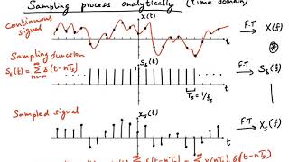
A continuous-time signal x(t) is represented as a sequence of discrete-time samples x[n] when sampled at a uniform rate fs (samples per second).
Detailed Explanation
This chunk defines the fundamental relationship between continuous-time and discrete-time signals. A continuous-time signal, denoted as x(t), refers to a signal that has values defined for every instant in time. In contrast, when this signal is sampled at regular intervals, it transforms into a discrete-time signal, denoted as x[n]. This means that instead of having information at every moment, we only consider specific points or samples, determined by a fixed sampling rate, fs (the number of samples taken per second).
Examples & Analogies
Imagine watching a video versus looking at a flipbook. The video shows fluid motion (like the continuous-time signal), while the flipbook, made of individual pages turned quickly, gives you the impression of motion, but only at discrete intervals (like the discrete-time signal). Each page in the flipbook corresponds to a sample of the video at a specific time.
Sampling Period and Frequency
Chapter 2 of 2
🔒 Unlock Audio Chapter
Sign up and enroll to access the full audio experience
Chapter Content
The discrete-time signal is given by: x[n] = x(nT) where:
- T is the sampling period, T = 1/fs, and fs is the sampling frequency.
- x[n] is the value of the continuous signal at time t = nT, where n is an integer.
Detailed Explanation
This chunk elaborates on the mathematical representation of discrete-time signals. It introduces the formula x[n] = x(nT), where T represents the sampling period—the time interval between each sample. This means every n-th sample corresponds to the continuous signal's value at a specific time calculated as nT, with n being an integer (0, 1, 2, ...). Furthermore, T is inversely related to the sampling frequency fs, emphasizing that a higher sampling frequency results in a lower sampling period and vice versa.
Examples & Analogies
Think of a clock. If the clock ticks once every second, that would be your sampling frequency of 1 Hz, and the T would be 1 second. If you were to record the time every tick (or every second), you would essentially be sampling the passage of time in a discrete manner, just like how one samples a continuous signal.
Key Concepts
-
Sampling: The process of converting a continuous-time signal into discrete-time by capturing values at fixed intervals.
-
Discrete-Time Signal Representation: The mathematical relationship between continuous-time signals and sequences of samples.
Examples & Applications
If a continuous signal x(t) is sampled every 0.01 seconds, the discrete-time representation could be x[n] = x(n * 0.01) where n = 0, 1, 2, ...
A signal with frequencies up to 500 Hz must be sampled at least at 1,000 Hz to avoid aliasing, as per the Nyquist theorem.
Memory Aids
Interactive tools to help you remember key concepts
Rhymes
To keep the signal clear, sample twice as fast, or you'll face aliasing, which can be a problem vast.
Stories
Imagine a painter who wants to capture every detail of a landscape. If he only paints it every few minutes, he might miss out on changes. Similarly, sampling captures details of a signal over time at specific intervals. If done too sparsely, details get lost or misrepresented.
Memory Tools
T = 1/fs can be remembered as 'Time is the inverse of frequency'.
Acronyms
For aliasing, remember AVOID
Always Verify that Overlapping Interferes with Discrete signals.
Flash Cards
Glossary
- DiscreteTime Signal
A representation of a signal defined only at distinct intervals, typically created by sampling a continuous-time signal.
- Sampling Period (T)
The time interval between consecutive samples in a sampling process.
- Sampling Frequency (fs)
The number of samples taken per second, defined as fs = 1/T.
- Aliasing
A phenomenon that occurs when a signal is sampled below its Nyquist rate, leading to misinterpretation of frequencies.
- Nyquist Rate
The minimum sampling frequency required to avoid aliasing, which is twice the maximum frequency present in the signal.
Reference links
Supplementary resources to enhance your learning experience.