
Local Equilibrium Assumption
Enroll to start learning
You’ve not yet enrolled in this course. Please enroll for free to listen to audio lessons, classroom podcasts and take practice test.
Interactive Audio Lesson
Listen to a student-teacher conversation explaining the topic in a relatable way.
Introduction to Local Equilibrium
🔒 Unlock Audio Lesson
Sign up and enroll to listen to this audio lesson

Today, we'll explore the local equilibrium assumption, a crucial concept in environmental engineering. What happens to contaminants when they interact with sediments?

Are we saying that they just settle in the sediments without changing?
Good question! It's more nuanced. The local equilibrium assumption posits that the rates of diffusion of contaminants in water and their adsorption onto sediments reach an equilibrium.

So, does this mean that everything is always balanced in that moment?
Exactly! This temporary balance enables us to model the behavior but only under specific conditions—like low water movement.

And if there's a strong flow? Would that mean the equilibrium doesn't hold?
Precisely! That's why we need different approaches when advection is significant.
Let's summarize: The local equilibrium assumption tells us how solutes interact dynamically in sediments, enabling effective modeling of contaminant transport.
Mathematical Expression of the Assumption
🔒 Unlock Audio Lesson
Sign up and enroll to listen to this audio lesson

Let's delve into the mathematics behind this. Can someone remind me how we express the concentration relationship between the solid and liquid?

It's the linear expression with the partition coefficient, right?
Correct! We can say: `C_s = K_d * C_l`. How does this help us in our evaluations?
It simplifies understanding of the distribution between phases!
Absolutely. This equation allows us to calculate how much of a solute exists in solid compared to the liquid.
Does this mean we can predict the effective diffusion as well?
Yes, knowing these concentrations leads to calculating the retardation factor, a critical value in determining the speed of contaminant spread.
Summarizing, the linear relationship helps us relate solid and liquid concentrations, vital for modeling effects in environmental systems.
When Does the Assumption Fail?
🔒 Unlock Audio Lesson
Sign up and enroll to listen to this audio lesson
Now, let's discuss when our assumption might break down. Can anyone think of a scenario?
If the flow of water is too fast?
Exactly! High water velocity can disrupt equilibrium. What implications does that have?
It means we'll need a more complex model that includes transient behaviors!
Spot on! As a result, the solute may not have enough time to adsorb onto the solids. What’s one way we can adjust our models?
We could factor in the mass transport equations to describe the advection-diffusion dynamics better.
Exactly! When modeling these systems, transitioning to a non-equilibrium framework can provide a more accurate representation of behavioral changes.
To conclude, recognizing the limitation of the local equilibrium assumption is crucial for accurate environmental modeling.
Introduction & Overview
Read summaries of the section's main ideas at different levels of detail.
Quick Overview
Standard
This section discusses the local equilibrium assumption, which posits that diffusion and adsorption processes reach a near-instantaneous balance at each point in a heterogeneous medium. The relationship established between the concentration of a solute in the liquid phase and its counterpart in the solid phase allows for practical modeling in environmental engineering.
Detailed
Detailed Summary
The local equilibrium assumption is a pivotal concept in environmental engineering, specifically when evaluating the interactions between solid particles and pore water in porous media. This assumption postulates that the rates of diffusion and adsorption/desorption equilibrate quickly at any given point within the system.
Key Points:
- Equilibrium in Diffusion and Adsorption: The assumption relies on the notion that the rate of chemical movement through diffusion is of the same order of magnitude as the rate of adsorption. Hence, at each point of interest, the distribution of solutes can be regarded as reaching equilibrium almost instantaneously.
- Formulation: Mathematically, this is expressed with the assumption that the concentration of a solute in the solid phase is linearly related to its concentration in the fluid phase (represented as:
,
where C_s is the concentration in the solid phase, C_l is the concentration in the liquid phase, and K_d is a linear distribution coefficient).
- Conditions for Validity: The local equilibrium assumption holds true when the velocity of water movement (advection) is relatively low compared to the rates of adsorption/desorption. Should advection surpass these rates, the assumption would no longer be appropriate, requiring modification of the model to consider transient conditions.
- Retardation Factor: The equilibrium leads to the calculation of the effective diffusivity which is influenced by factors like porosity and the bulk density of solids, impacting the overall diffusion rate observed in such systems. This results in formulating retardation factors that account for the interplay between adsorption and diffusion in model equations.
-
Application: In practice, understanding the local equilibrium allows environmental engineers to simulate and predict contaminant transport in sediment-water systems effectively.
In essence, while the local equilibrium assumption is a simplification, it provides critical insights into the dynamics of chemical interactions within environmental systems.
Youtube Videos


Audio Book
Dive deep into the subject with an immersive audiobook experience.
Introduction to the Local Equilibrium Assumption
Chapter 1 of 4
🔒 Unlock Audio Chapter
Sign up and enroll to access the full audio experience
Chapter Content
this we will invoke what is called as a local equilibrium assumption. These are all simplifications for what could be the real scenario what is happening in the system. Local equilibrium assumption assumes that when a solid is near a fluid, there are these chemicals that are sitting here we and there is chemical here, the rate at which the diffusion is occurring is almost the same order of magnitude at which this adsorption is happening.
Detailed Explanation
The local equilibrium assumption suggests that when a solid and a fluid are in close proximity, the rate of diffusion of substances between them and the rate of adsorption onto the solid are balanced. In simpler terms, this means that for every molecule that moves from the fluid to the solid, a molecule would move back from the solid to the fluid at a similar rate. Therefore, we can assume that the system is in a state of equilibrium — where concentrations of solute molecules in both phases remain stable over time.
Examples & Analogies
Think of a busy highway where cars are merging from a side road. If the side road has a flow of cars merging onto the highway that is equal to the number of cars exiting the highway back onto the side road, the number of cars on the highway stays relatively constant. Similarly, in a localized area where a solid is in contact with a fluid, chemicals are in constant motion balancing their concentration.
Conditions for Equilibrium
Chapter 2 of 4
🔒 Unlock Audio Chapter
Sign up and enroll to access the full audio experience
Chapter Content
So, which means this is diffusion. Here also can be diffusion, the mass transfer coefficient associated with the adsorption is also diffusion, there is no flow anywhere, so everything is diffusion.
Detailed Explanation
For the local equilibrium assumption to hold, the only mode of transport involved should be diffusion — meaning that there isn't any bulk flow in the system. In this scenario, all interactions between the molecules in the solid phase and those in the fluid phase occur through diffusion. Therefore, the assumption of equilibrium can be validated if the mass transfer processes through adsorption do not involve rapid fluid flows, as these would disrupt the equilibrium.
Examples & Analogies
Imagine a sponge in a bowl of water. Initially, the sponge absorbs water through soft, gradual soakage (diffusion). If you suddenly pour in more water or stir the bowl (inducing flow), the equilibrium is disrupted. The sponge's ability to absorb and release water is based on the slow and steady process of diffusion rather than chaotic flow.
Importance of Rate Equivalence
Chapter 3 of 4
🔒 Unlock Audio Chapter
Sign up and enroll to access the full audio experience
Chapter Content
Therefore, this scale of this one is equivalent to the rate at which this is happening.
Detailed Explanation
The local equilibrium assumption relies on the idea that the rates of diffusion into the solid and out of the solid are equivalent. If diffusion into the solid is significantly faster than diffusion out of the solid, equilibrium cannot truly exist. This rate equivalence is fundamental, as it simplifies the mathematical modeling of processes like adsorption and desorption in environmental systems. Essentially, the quicker these processes can be assumed to occur in tandem, the easier it becomes to analyze and predict the interactions at play.
Examples & Analogies
Consider a balance scale where two weights, one on each side, maintain the balance. If you add weight to one side without compensating the other, the scale tips, disrupting the balance. In a similar manner, if the diffusion rates are unbalanced, you cannot assume that a stable equilibrium exists between a solid and fluid system.
Practical Implications of the Assumption
Chapter 4 of 4
🔒 Unlock Audio Chapter
Sign up and enroll to access the full audio experience
Chapter Content
If my diffusion occurring in a simple tube, the equation will be normal diffusion equation.
Detailed Explanation
If we assume that the local equilibrium condition is met, we can use simpler equations to model diffusion in systems. Specifically, in the absence of complex flow dynamics, the simple diffusion equation applies, allowing us to predict how substances will move over time. This leads to predictions about contamination spread, pollutant transport, and general mass transfer efficiencies within environmental systems. However, recognizing real-world deviations from this assumption is crucial for accurate predictions.
Examples & Analogies
Think of a water fountain's spray, where water travels upward then falls back down in a predictable pattern. If you were to analyze how water moves using simple physics equations, you’d be pleasantly surprised at how much you can predict. But if you throw a handful of dried leaves into the water, they create a swirl and disrupt the simple pattern, complicating predictions. Just like in fluid dynamics, local equilibrium allows for simplicity, but real-world complications can emerge.
Key Concepts
-
Local Equilibrium Assumption: The simplifying hypothesis that allows for the modeling of solute interaction in porous media under specific conditions.
-
Diffusion: The process by which solutes move across a concentration gradient.
-
Retardation Factor: A factor that indicates how solids impact the diffusion rate of solutes.
Examples & Applications
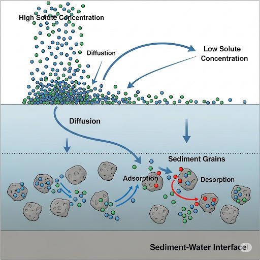
The local equilibrium assumption in action can be observed in sediments where pollutants diffuse and equilibrate with solid particles.
If the water flow increases, such as during a heavy rainfall, the local equilibrium may not be maintained, requiring adjusted modeling strategies.
Memory Aids
Interactive tools to help you remember key concepts
Rhymes
In sediment's hold, contaminants fade, / Equilibrium's balance, solutes invade.
Stories
Imagine a busy riverbank where water flows slowly over sand and stone. The pollutants dip in and out, finding their homes in solid grains, all while maintaining a delicate dance of equilibrium.
Memory Tools
EASY - Equilibrium and Adsorption Same Yield: A mnemonic to remember the quick balance between liquid and solid phases.
Acronyms
L.E.A.P. - Local Equilibrium Assumption Principle.
Flash Cards
Glossary
- Local Equilibrium Assumption
The hypothesis that diffusion and adsorption processes quickly reach a balance at every point in a porous medium.
- Diffusion
The movement of particles from an area of higher concentration to an area of lower concentration.
- Adsorption
The process of accumulating a substance on the surface of a solid.
- Retardation Factor
A dimensionless number that quantifies how the presence of solid materials slows down the diffusion of solutes.
- Partition Coefficient (K_d)
A constant that describes the ratio of solute concentration in the solid phase to that in the liquid phase at equilibrium.
Reference links
Supplementary resources to enhance your learning experience.