
Control Volume Approach for Unsteady Flow
Enroll to start learning
You’ve not yet enrolled in this course. Please enroll for free to listen to audio lessons, classroom podcasts and take practice test.
Interactive Audio Lesson
Listen to a student-teacher conversation explaining the topic in a relatable way.
Introduction to Control Volume Approach
🔒 Unlock Audio Lesson
Sign up and enroll to listen to this audio lesson

Today, we will delve into the control volume approach within unsteady flow analysis. Can anyone tell me why this approach might be useful in fluid mechanics?

I think it helps us break down complex flows into manageable parts.
Exactly! The control volume approach allows us to apply conservation laws effectively. Remember, fluid mechanics often requires us to analyze systems that change over time. Now, what do we mean by unsteady flows?

Unsteady flows have properties that change with time, right?
Correct! And that leads us to the Reynolds transport theorem. It is fundamental when transitioning from systems to control volumes. Can anyone describe its significance?

It connects the physical quantities we measure in a system with those we compute in a control volume.
Exactly! The theorem is a bridge from theoretical to practical application.
Let's summarize: the control volume approach simplifies the analysis of unsteady flows while the Reynolds transport theorem integrates our conservation principles. Great start!
Distinguishing Between Flow Types
🔒 Unlock Audio Lesson
Sign up and enroll to listen to this audio lesson

Next, let's clarify the types of flow we will be discussing. Who can define compressible versus incompressible flow for me?

Incompressible flow means the fluid density is constant while compressible flow can change with pressure and temperature.
Perfect! Compressible flows are typically found in gases under high-pressure variations. Why might we prefer to simplify our problems to incompressible flow?
Because it allows us to drop certain terms in our equations, making calculations simpler.
Exactly! Simplifying to incompressible flow lets us focus more on the velocity field and pressure without worrying about density fluctuations. Now, let’s apply these concepts to a problem.
To recap, recognizing the type of flow significantly impacts the equations we derive and the methods we use. This foundational understanding is crucial for effective engineering solutions.
Linear Momentum Equations
🔒 Unlock Audio Lesson
Sign up and enroll to listen to this audio lesson
Now let's discuss linear momentum equations derived from the control volume approach. Can someone remind me why momentum is important in fluid mechanics?
Momentum helps us understand forces acting on fluids, which is essential for engineering applications like pipe flows.
Exactly! To derive our equations, let's consider a control volume in motion. We’ll take into account both surface and body forces acting on the fluid. Who remembers the types of forces we consider?
Surface forces include pressure and viscous forces, while body forces include gravity.
Right! The balance of these forces allows us to describe the momentum change within the control volume. Let’s say we have inflow and outflow; how does that factor in?
We must account for the flow rates entering and leaving to apply conservation principles accurately.
Absolutely! Balancing these equations enables us to derive useful insights into fluid behavior under various conditions.
In summary, understanding the linear momentum equations equips us with the tools to predict fluid interactions based on fundamental laws of dynamics. Excellent job today!
Applications and Real-World Examples
🔒 Unlock Audio Lesson
Sign up and enroll to listen to this audio lesson
Finally, let's look at some real-world applications where the control volume method is beneficial. Can anyone think of a scenario where this approach is vital?
Designing hydraulic systems in civil engineering!
Or managing water distributions in reservoirs.
Exactly! Each example requires an understanding of how fluid behavior can change under different conditions. Let's solve a problem related to water flow through a dam, which uses similar principles.
Would we use the same equations we derived before?
Yes! We take the same theoretical framework and apply it to assess performance and safety in a hydraulic structure.
To conclude this session, remember that understanding the principles we discussed allows for efficient and safe designs in engineering projects.
Introduction & Overview
Read summaries of the section's main ideas at different levels of detail.
Quick Overview
Standard
The section elaborates on the application of the control volume approach for unsteady flow based on the Reynolds transport theorem. It emphasizes the simplifications for steady and unsteady conditions, delineates between compressible and incompressible flows, and introduces key concepts such as momentum flux correction factor, exemplifying these through practical problems and applications.
Detailed
Control Volume Approach for Unsteady Flow
The control volume approach is a vital tool in fluid mechanics for understanding the behavior of fluid flow over time. In this section, we explore the application of this approach to unsteady flow scenarios, leveraging the Reynolds transport theorem as the foundation.
Key Concepts Covered
- Reynolds Transport Theorem: It's essential for joining the principles of conservation of mass and momentum to real-world applications in fluid systems.
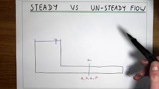
- Unsteady vs. Steady Flow: The section clarifies how unsteady and steady flows differ, emphasizing that steady conditions simplify the application of the Reynolds transport theorem.
- Flow Types: Differentiating between compressible and incompressible fluid flows, as well as one-dimensional versus multi-dimensional flow contexts.
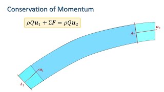
- Conservation of Momentum: We derive the linear momentum equations for both fixed and moving control volumes. These equations are crucial for predicting forces acting on the fluid.
- Practical Examples: Various examples demonstrate how to apply these equations to real-world problems, solidifying the understanding of theoretical concepts through practical application.
In conclusion, this section highlights the interplay between conservation laws and practical fluid dynamics, guiding engineers to design systems like dams and pipelines effectively.
Youtube Videos
![System Approach and Control Volume Approach [Fluid Mechanics]](https://img.youtube.com/vi/quK9rvsZTPA/mqdefault.jpg)


Audio Book
Dive deep into the subject with an immersive audiobook experience.
Introduction to Control Volume Approach
Chapter 1 of 5
🔒 Unlock Audio Chapter
Sign up and enroll to access the full audio experience
Chapter Content
In fluid mechanics, the control volume approach is a critical method for analyzing fluid flow. It allows for the application of fundamental equations to understand how fluid behavior changes over time and space.
Detailed Explanation
The control volume approach involves defining a specific region in space (the control volume) through which fluid flows. By applying the conservation of mass, momentum, and energy principles within this volume, we can determine how the fluid characteristics change over time. The key is to focus on the flow across the boundaries of the volume, accounting for inflows and outflows.
Examples & Analogies
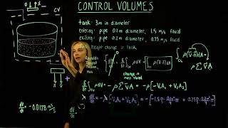
Imagine a water tank with an inlet pipe filling it and an outlet pipe draining it. The tank acts as a control volume. By measuring the flow rates at the inlet and outlet, we can predict the water level in the tank over time, thus understanding how the system behaves under different conditions.
Unsteady Flow Concept
Chapter 2 of 5
🔒 Unlock Audio Chapter
Sign up and enroll to access the full audio experience
Chapter Content
Unsteady flow refers to a condition where the fluid characteristics (like velocity or pressure) change with time at a given point. This is different from steady flow, where these properties remain constant over time.
Detailed Explanation
In unsteady flow situations, the equations that govern the conservation of mass, momentum, and energy need to take into account the changes that occur over time. As properties change, we cannot assume that the fluid behaves uniformly throughout the control volume or along the boundaries.
Examples & Analogies
Consider a bathtub draining. Initially, the water level drops quickly, but as the tub empties, the rate of change slows. This exemplifies unsteady flow because the water level (a property of the fluid) changes at different rates over time until the tub is empty.
Application of Reynolds Transport Theorem
Chapter 3 of 5
🔒 Unlock Audio Chapter
Sign up and enroll to access the full audio experience
Chapter Content
The Reynolds transport theorem provides a framework to relate the rate of change of a property within the control volume to the flow of that property across the control volume's boundaries.
Detailed Explanation
The theorem states that the change in a fluid property (such as mass or momentum) in a control volume can be expressed as the sum of the changes within the volume itself and the flux of that property across the boundaries. This is particularly useful for deriving equations of motion for unsteady flows as it connects the local changes in a fluid with the flow entering or exiting the control volume.
Examples & Analogies
Think of a sponge. When you squeeze it, you release water (property) out of the sponge and simultaneously, if you submerge it in water, it absorbs some, changing the amount of water it holds. Here, the sponge acts like your control volume, with water being the property whose rate of change we’re tracking.
Equations for Unsteady Flow
Chapter 4 of 5
🔒 Unlock Audio Chapter
Sign up and enroll to access the full audio experience
Chapter Content
In unsteady flow conditions, the equations representing conservation principles must be adapted to account for the time-dependent changes. This involves using partial derivatives to express the rate of change over time.
Detailed Explanation
The equations governing unsteady flow involve partial derivatives that capture how the fluid properties change with respect to time. This includes terms for mass influx and efflux across the boundaries and the time-variant characteristics of the fluid within the control volume. The complexity can increase based on whether the flow is compressible or incompressible.
Examples & Analogies
Consider a water reservoir filling and emptying simultaneously, where we want to calculate how full it is after a certain time. The changing levels require us to account for both inflow (the supply of water) and outflow (the drainage). This time-dependent nature makes the situation reflect unsteady flow.
Momentum Flux Correction Factor
Chapter 5 of 5
🔒 Unlock Audio Chapter
Sign up and enroll to access the full audio experience
Chapter Content
The momentum flux correction factor is introduced to account for varying velocity profiles across the control volume's cross-sectional area, especially in cases of non-uniform flow.
Detailed Explanation
In fluid flow, the velocity is not constant across a cross-section of a pipe or channel. The momentum flux correction factor adjusts the momentum equation to accurately reflect the actual flow conditions by incorporating the effects of velocity distribution on momentum exchange.
Examples & Analogies
Imagine the wind blowing through a tree. The branches closer to the trunk experience more wind than the leaves at the tips. If we want to calculate the force exerted by the wind on the tree, we must consider this variation in wind speed across different parts, similar to how the momentum flux correction factor adjusts calculations for non-uniform velocity profiles.
Key Concepts
-
Reynolds Transport Theorem: It's essential for joining the principles of conservation of mass and momentum to real-world applications in fluid systems.
-
Unsteady vs. Steady Flow: The section clarifies how unsteady and steady flows differ, emphasizing that steady conditions simplify the application of the Reynolds transport theorem.
-
Flow Types: Differentiating between compressible and incompressible fluid flows, as well as one-dimensional versus multi-dimensional flow contexts.
-
Conservation of Momentum: We derive the linear momentum equations for both fixed and moving control volumes. These equations are crucial for predicting forces acting on the fluid.
-
Practical Examples: Various examples demonstrate how to apply these equations to real-world problems, solidifying the understanding of theoretical concepts through practical application.
-
In conclusion, this section highlights the interplay between conservation laws and practical fluid dynamics, guiding engineers to design systems like dams and pipelines effectively.
Examples & Applications
Calculating flow rates within a pipe system during varying flow conditions.
Examining the impact of inflow and outflow on fluid storage within reservoirs.
Memory Aids
Interactive tools to help you remember key concepts
Rhymes
Control volume, steady or not, fluids flowing in, they can't be caught.
Stories
Imagine a river where water levels rise and fall. Analyzing what goes in and out at different times helps us manage the flow, like managing a bank account for water.
Memory Tools
For 'R' in Reynolds, think 'Relate' – it connects systems to control volumes.
Acronyms
FLOW - Fluid Laws Of Conservation in the context of the control volume approach.
Flash Cards
Glossary
- Reynolds Transport Theorem
A theorem that relates the time rate of change of a quantity in a control volume to the flow of that quantity across the boundary of the control volume.
- Control Volume
A defined region in space through which fluid may flow in and out.
- Incompressible Flow
Flow in which the fluid density is constant throughout.
- Compressible Flow
Flow where fluid density changes significantly, often due to pressure or temperature variations.
- Conservation of Momentum
A principle stating that the total momentum of a closed system remains constant unless acted upon by an external force.
Reference links
Supplementary resources to enhance your learning experience.