
Continuity Equations
Enroll to start learning
You’ve not yet enrolled in this course. Please enroll for free to listen to audio lessons, classroom podcasts and take practice test.
Interactive Audio Lesson
Listen to a student-teacher conversation explaining the topic in a relatable way.
Basic Concept of Continuity Equations
🔒 Unlock Audio Lesson
Sign up and enroll to listen to this audio lesson

Today we will discuss continuity equations, focusing on how we can express mass conservation in fluid mechanics. Can anyone tell me what mass conservation means?

I think mass conservation means that the mass in a closed system doesn't change over time.
Exactly! In fluid mechanics, we translate this idea into mathematical equations, specifically continuity equations. Let’s explore how this applies to infinitesimally small control volumes. Why do we consider control volumes that are infinitely small?

Because it helps us analyze the flow and changes in mass more easily at a local level!
Great observation! By focusing on infinitesimal control volumes, we can formulate the differential form of the mass conservation equation.
Remember the acronym **DIV** to recall how divergence plays a crucial role in our computations, as we represent mass changes using the divergence of mass flux.
In summary, mass conservation in fluid mechanics is encapsulated in continuity equations revealing how mass flows through control volumes.
Application of the Gauss Theorem
🔒 Unlock Audio Lesson
Sign up and enroll to listen to this audio lesson

Now let’s delve into how the Gauss theorem helps us derive these equations. Can anyone explain what Gauss's theorem states?

I believe it relates the flow of a quantity through a surface to the divergence of that quantity within the volume.
Right! This relationship is foundational for deriving our continuity equations. Now, when we apply this to control volume analysis, what variables do we need to consider?

We need to consider density and velocity fields!
Exactly, both density (ρ) and velocity (v) are essential. We can express them as functions of space and time. Using Taylor series, we can approximate them at different control surface points. Does anyone remember why we use Taylor series here?
It helps us estimate the function’s behavior at various points using its value and derivatives at a single point.
Correct! This approximation leads us to the final forms of our continuity equations, balancing the change in mass within the control volume with the mass flux across its surface.
Exploring Compressible and Incompressible Flows
🔒 Unlock Audio Lesson
Sign up and enroll to listen to this audio lesson
Let’s discuss the implications of mass conservation in different types of flows. What are the key differences between compressible and incompressible flows?
Incompressible flows assume constant density, while compressible flows can have varying density.
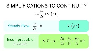
Exactly! For incompressible flow, the divergence of the velocity field equals zero. What happens in compressible flow scenarios?
In compressible flows, the density changes, and we have to account for those changes in our continuity equations.
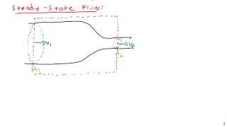
That’s right! We often see compressible flows in high-speed applications, like gas dynamics, whereas incompressible flows are common in water and low-speed applications. Remember, under steady-state flow conditions, there will be no change in mass within a control volume for both types!
In summary, understanding the differences between compressible and incompressible flows allows us to properly apply continuity equations in various scenarios.
Application and Limitations of Continuity Equations
🔒 Unlock Audio Lesson
Sign up and enroll to listen to this audio lesson
Now that we’ve covered the foundational aspects, let’s talk about where we apply these continuity equations in real-world problems. Can anyone provide examples?
We can apply them in pipe flow problems and in designing various hydraulic systems!
Great examples! However, are there scenarios where these equations might not apply properly?
If the flow is turbulent or if we have compressible flows, the assumptions might not hold true.
Exactly! While continuity equations simplify many problems, complex flow conditions or drastic changes in fluid properties can challenge their applicability.
In summary, while continuity equations are powerful, understanding their limitations in various contexts is equally essential for accurate analysis.
Introduction & Overview
Read summaries of the section's main ideas at different levels of detail.
Quick Overview
Standard
Continuity equations serve as fundamental tools in fluid mechanics to express mass conservation. By analyzing infinitesimal control volumes, the section delves into differential forms of mass conservation equations derived from principles like the Gauss theorem, incorporating both density and velocity fields in Cartesian coordinates.
Detailed
Continuity Equations
Continuity equations are crucial in fluid mechanics as they express mass conservation within fluid systems. This section begins by discussing the concept of mass conservation through infinitely small control volumes defined by dimensions B4x, B4y, and B4z approaching zero. The primary goal is to form differential equations that encapsulate this principle.
Key components of continuity equations include:
- Density Field (ρ): Represented as a scalar function of position (x, y, z) and time (t).
- Velocity Field (v): Expressed as a vector field with components (u, v, w) dependent on space and time.
Utilizing Gauss's theorem, the section derives the differential equations indicating how mass storage changes within a control volume is equalized with the net mass outflux across control surfaces. The net outflux is described by the divergence of mass flux (ρv). The section also simplifies the analysis by employing Taylor series expansions to approximate velocity fields at different faces of the control volume and derives the final continuity equation form.
Through examples, the section highlights differences between incompressible and compressible flow, ultimately reinforcing the conditions under which mass conservation principles apply effectively.
Youtube Videos


Audio Book
Dive deep into the subject with an immersive audiobook experience.
Introduction to Continuity Equations
Chapter 1 of 6
🔒 Unlock Audio Chapter
Sign up and enroll to access the full audio experience
Chapter Content
Continuity equations are essentially mass conservation equations for infinitely small control volumes. This means we consider control volumes that are infinitesimally small, leading to a differential equations format for mass conservation.
Detailed Explanation
Continuity equations encapsulate the principle of mass conservation, indicating that mass cannot simply vanish or appear without cause. By examining very small sections of a flow (control volumes), we can derive mathematical relationships that describe how mass changes over time within these volumes. Using these relationships allows engineers to predict how fluids behave in various conditions.
Examples & Analogies
Think of a water jug. If you pour water in (mass influx) and it starts evaporating (mass outflux), the amount of water in the jug changes. The continuity equation helps to mathematically describe this change and ensure that the water conserves mass in the jug.
Density and Velocity Fields in Control Volumes
Chapter 2 of 6
🔒 Unlock Audio Chapter
Sign up and enroll to access the full audio experience
Chapter Content
In our equations, rho represents the density field, which is a scalar function dependent on positions x, y, z. The velocity field v consists of components u, v, w, which are also functions of positions x, y, z, and time.
Detailed Explanation
Density (rho) quantifies how much mass is present in a given volume of fluid, while the velocity field (represented as v) describes how fast and in what direction the fluid is moving. Understanding both the density and velocity fields is crucial because they directly influence how fluid flows through different environments.
Examples & Analogies
Imagine traffic on a highway. The density of cars in a section of the highway (how many cars are present per mile) and their velocities (how fast they are moving) are crucial for determining how congested it will be and how smoothly traffic will flow.
Using Gauss's Theorem for Mass Flow
Chapter 3 of 6
🔒 Unlock Audio Chapter
Sign up and enroll to access the full audio experience
Chapter Content
By applying Gauss's theorem, we can derive equations indicating the change in mass within control volumes and compare this to the mass flux entering or leaving the volume.
Detailed Explanation
Gauss's theorem helps relate the flow of mass into and out of a control volume to the change of mass stored within that volume. By integrating over the control volume's surface, we can quantify how much mass is entering versus how much is leaving. This is essential for ensuring that the mass is conserved.
Examples & Analogies
Consider a balloon being inflated. The air (mass) flowing into the balloon needs to equal the volume of air (mass) that stays inside the balloon. If more air flows in than what can be held, the balloon will eventually burst. The equations from Gauss’s theorem help predict these kinds of conditions.
Deriving Mass Conservation Equations
Chapter 4 of 6
🔒 Unlock Audio Chapter
Sign up and enroll to access the full audio experience
Chapter Content
To derive mass conservation equations for infinitesimally small control volumes, we consider how mass enters and exits through various surfaces and assume steady state conditions.
Detailed Explanation
By simplifying our control volumes to very small dimensions, we can apply Taylor series expansions to better predict how mass changes occur. This involves assuming that the velocity and density don't change dramatically within the space of our small control volume. The equations can then be simplified by canceling out negligible higher-order terms.
Examples & Analogies
Imagine measuring water flow through a narrow glass tube. If the tube is very narrow and you're only observing a small segment, any changes in water level might be so small that they can be ignored, simplifying the calculations you need to make.
Total Volume and Mass Flow Rate Calculations
Chapter 5 of 6
🔒 Unlock Audio Chapter
Sign up and enroll to access the full audio experience
Chapter Content
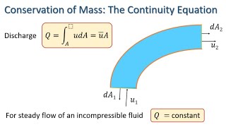
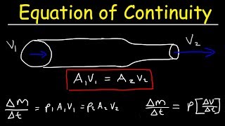
We express the net mass flow rate into a control volume as the difference between mass fluxes entering and leaving the volume, considering all three spatial directions.
Detailed Explanation
The total mass flow into a control volume can be calculated by considering the mass flowing in through each side of the volume. By subtracting the mass flow rate out from the mass flow rate in, we can determine how mass changes over time within that control volume.
Examples & Analogies
Think of filling a bathtub. The flow of water from the tap (inflow) needs to be greater than the outflow from the drain for the water level to rise. By knowing both the inflow and outflow rates, you can predict when the tub will overflow.
Final Equation and Interpretation
Chapter 6 of 6
🔒 Unlock Audio Chapter
Sign up and enroll to access the full audio experience
Chapter Content
Ultimately, through all these calculations and simplifications, we arrive at a final equation representing the conservation of mass in fluid mechanics, which can be noted as the divergence of the mass flux equal to the change in mass storage.
Detailed Explanation
The final compact form of the continuity equation helps us track how mass behaves through a control volume, allowing us to simplify complex flow conditions into manageable calculations. It essentially states that any changes in mass must be accounted for by the flow of mass into or out of a system.
Examples & Analogies
Consider an ice cream truck on a hot day. If more customers are buying ice cream (mass entering the truck's supply) than what the truck can replenish (mass leaving), the truck will eventually run out of ice cream. The continuity equation helps understand when that might happen.
Key Concepts
-
Mass Conservation: The principle stating that mass cannot be created or destroyed in a closed system.
-
Control Volume: A specific volume in space through which fluid flows, helping in the analysis of fluid properties.
-
Divergence of Mass Flux: Mathematical representation of how mass outflow and inflow interact in a defined control volume.
Examples & Applications
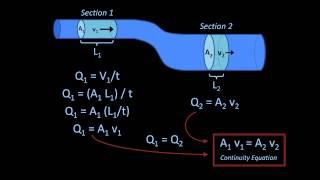
In industrial applications, continuity equations help in designing efficient piping systems by ensuring mass conservation.
In aerodynamics, analyzing airflow around objects utilizes continuity equations to predict pressure and velocity changes.
Memory Aids
Interactive tools to help you remember key concepts
Rhymes
In fluid flow where mass prevails, Conservation’s key in all scales.
Stories
Imagine a river flowing through a valley. The amount of water that flows in and out remains the same over time, reminding us of mass conservation.
Memory Tools
Do Not Vary - Divergence of Density Varies.
Acronyms
DICE - Divergence Indicates Change in Energy.
Flash Cards
Glossary
- Continuity Equation
An equation that describes the transport of some quantity in a system, particularly mass conservation in fluid dynamics.
- Control Volume
A defined space through which fluid flows, used to analyze mass and energy transfer.
- Divergence
A measure used in vector calculus that describes the rate of change of a quantity’s volume density in space.
- Compressible Flow
Flow where the fluid density changes significantly with pressure or temperature variations.
- Incompressible Flow
Flow where the fluid density is constant, regardless of pressure changes.
- Gauss Theorem
A fundamental theorem in vector calculus relating the divergence of a vector field to the flow across a closed surface.
Reference links
Supplementary resources to enhance your learning experience.