
Diagonalization
Enroll to start learning
You’ve not yet enrolled in this course. Please enroll for free to listen to audio lessons, classroom podcasts and take practice test.
Interactive Audio Lesson
Listen to a student-teacher conversation explaining the topic in a relatable way.
Introduction to Diagonalization
🔒 Unlock Audio Lesson
Sign up and enroll to listen to this audio lesson

Today, we'll discuss diagonalization. Diagonalization allows us to express a square matrix as a product involving a diagonal matrix, making computations simpler. Can anyone tell me why simplifying a matrix is useful?

It makes calculus with matrices easier, right? Like when you want to raise a matrix to a power.
Exactly! By diagonalizing a matrix A into PDP⁻¹, we can easily compute A^k = PD^kP⁻¹. This is a major advantage in applications, especially in civil engineering. Now, what does P and D represent?

P consists of eigenvectors, and D has eigenvalues along its diagonal?
Correct! Remember the acronym 'PEB' - P for eigenvectors, E for eigenvalues in D, and B for simpler computations! Let's move on to how we find these eigenvalues and eigenvectors.
Finding Eigenvalues and Eigenvectors
🔒 Unlock Audio Lesson
Sign up and enroll to listen to this audio lesson

To diagonalize a matrix, we need to find its eigenvalues first. Who can tell me the characteristic equation we solve to find these eigenvalues?

Is it det(A - λI) = 0?
Yes! Great job! Once we have the eigenvalues, the next step is to find the eigenvectors corresponding to each eigenvalue. How do we do that?

We solve the equation (A - λI)v = 0 for each eigenvalue?
Exactly! This process gives us the necessary eigenvectors we need. Remember the phrase 'Solve for v' to recall this step. Let’s discuss why having linearly independent eigenvectors is crucial.
Diagonalization Criteria
🔒 Unlock Audio Lesson
Sign up and enroll to listen to this audio lesson
Now, let's talk about the criteria for diagonalization. A matrix must have how many linearly independent eigenvectors to be diagonalizable?
It needs n linearly independent eigenvectors, right?
Yes! And if the algebraic and geometric multiplicities do not match for any eigenvalue, the matrix won't be diagonalizable. Who remembers what we mean by these multiplicities?
Algebraic multiplicity is how often the eigenvalue appears, and geometric is how many independent eigenvectors we find for it!
Exactly! Good memory! Let's summarize what we learned.
To recap, a matrix is diagonalizable if it has n linearly independent eigenvectors, and we've seen how to find these using eigenvalues. Also remember the special cases of distinct eigenvalues!
Introduction & Overview
Read summaries of the section's main ideas at different levels of detail.
Quick Overview
Standard
This section introduces the concept of diagonalization, stressing its importance in linear algebra and civil engineering. It covers the definitions of eigenvalues and eigenvectors, criteria for diagonalization, and the procedures involved in diagonalizing a matrix, complemented by practical applications in civil engineering.
Detailed
Detailed Summary
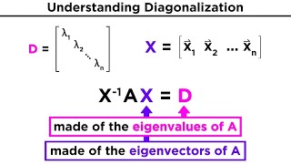
Diagonalization is a fundamental technique in linear algebra that aims to simplify computations involving square matrices by transforming them into diagonal matrices through similarity transformations. A matrix A is said to be diagonalizable if it can be represented as A = PDP⁻¹, where P is an invertible matrix of eigenvectors and D is a diagonal matrix of eigenvalues.
In order to diagonalize a matrix, one first finds its eigenvalues by solving the characteristic equation det(A − λI) = 0. The corresponding eigenvectors can then be determined by solving the equations (A - λI)v = 0 for each eigenvalue λ. A matrix is diagonalizable if it has as many linearly independent eigenvectors as its size indicates (n). Special cases such as distinct and repeated eigenvalues are discussed, highlighting that distinct eigenvalues guarantee diagonalizability while repeated ones may not.
The procedure for diagonalization is clearly outlined in steps, and an illustrative example with a 2x2 matrix is provided. The relevance of diagonalization extends to civil engineering, particularly in vibration analysis and structural dynamics, where the diagonalization of matrices leads to the decoupling of systems for simplified analysis. The section also briefly touches upon matrices that are not diagonalizable, introducing the Jordan form as a way to analyze them. Lastly, for symmetric matrices, important properties such as real eigenvalues and orthogonal eigenvectors are explained, showcasing their applicability in real-world engineering problems.
Youtube Videos


Audio Book
Dive deep into the subject with an immersive audiobook experience.
Introduction to Diagonalization
Chapter 1 of 5
🔒 Unlock Audio Chapter
Sign up and enroll to access the full audio experience
Chapter Content
Diagonalization is a powerful technique in linear algebra that simplifies matrix operations by converting a given square matrix into a diagonal matrix through similarity transformation. For civil engineers, diagonalization is particularly important in areas such as structural analysis, vibration analysis, and systems of differential equations. A diagonal matrix is easier to work with computationally, especially for raising a matrix to powers or solving systems of equations. Understanding when and how a matrix is diagonalizable allows engineers to interpret and simplify complex real-world models mathematically.
Detailed Explanation
Diagonalization is a method that transforms a complex square matrix into a simpler diagonal matrix, making calculations easier and more efficient. Engineers in fields like civil engineering benefit greatly from this because it helps them analyze structures, understand vibrations, and solve equations related to various structures. A diagonal matrix contains only eigenvalues on its diagonal, which simplifies the mathematics involved in matrix operations.
Examples & Analogies
Imagine you are trying to organize a jumble of books on a shelf. Instead of sorting through each book individually for details, you categorize them by genres and stack them neatly on the shelf. Diagonalization does something similar for matrices, organizing complex data into simpler, manageable forms (like genres) so that engineers can focus on the main points without being overwhelmed.
Diagonalization of a Matrix
Chapter 2 of 5
🔒 Unlock Audio Chapter
Sign up and enroll to access the full audio experience
Chapter Content
A square matrix A of order n×n is said to be diagonalizable if there exists an invertible matrix P and a diagonal matrix D such that: A=PDP−1 Here, • A is the original matrix, • D is the diagonal matrix, • P is the matrix whose columns are the linearly independent eigenvectors of A, • D contains the eigenvalues of A along its diagonal. This is called a similarity transformation, and it allows easier computation for powers of A: Ak =PDkP−1.
Detailed Explanation
A matrix A is diagonalizable if it can be expressed in the form A=PDP−1, meaning it can be rewritten using an invertible matrix P (formed from its eigenvectors) and a diagonal matrix D (containing its eigenvalues). This transformation makes it much easier to compute powers of A (like A^2, A^3, etc.) since you only need to raise the diagonal elements in D to the desired power and then perform simple multiplications.
Examples & Analogies
Think of diagonalizing a matrix like organizing a complex recipe into simpler steps. Instead of trying to manage all ingredients at once, you can work with each part (like chopping, mixing, and baking) separately. Once each step is done (akin to the diagonal matrix), you can then assemble the final dish (the full matrix operation).
Finding Eigenvalues and Eigenvectors
Chapter 3 of 5
🔒 Unlock Audio Chapter
Sign up and enroll to access the full audio experience
Chapter Content
To diagonalize a matrix, you must first find its eigenvalues and eigenvectors. Given an n×n matrix A, a non-zero vector ⃗v is called an eigenvector if: Av⃗=λv⃗ where λ is a scalar called the eigenvalue corresponding to ⃗v. To find eigenvalues: Solve det(A−λI)=0 This is called the characteristic equation. To find eigenvectors: • For each eigenvalue λ, solve the equation: (A−λI)⃗v=0.
Detailed Explanation
Before diagonalization can occur, we need to find the eigenvalues and eigenvectors of the matrix. Eigenvalues are scalar values that tell us how much an eigenvector is stretched or compressed during the transformation represented by the matrix. The eigenvalues are found by solving the characteristic equation, while the eigenvectors are determined by substituting each eigenvalue back into the matrix and solving for the respective vectors.
Examples & Analogies
Imagine you are a detective gathering clues (eigenvectors) about a particular case (matrix). You first need to identify significant evidence (eigenvalues) that leads you towards understanding the bigger picture. Once you have your evidence, you can put together a solid conclusion about what happened in the case, similar to how you form a diagonal matrix from your eigenvectors and eigenvalues.
Diagonalization Criteria
Chapter 4 of 5
🔒 Unlock Audio Chapter
Sign up and enroll to access the full audio experience
Chapter Content
A matrix A is diagonalizable if and only if: • It has n linearly independent eigenvectors. • Equivalently, the algebraic multiplicity (how many times an eigenvalue appears as a root of the characteristic polynomial) must equal the geometric multiplicity (dimension of the eigenspace) for each eigenvalue. Special Cases: • Distinct Eigenvalues: If all eigenvalues are distinct, then A is always diagonalizable. • Repeated Eigenvalues: Matrix may or may not be diagonalizable; check the number of linearly independent eigenvectors.
Detailed Explanation
For a matrix to be diagonalizable, it must have enough unique eigenvectors, specifically n linearly independent eigenvectors where n is the order of the matrix. If the eigenvalues are distinct, diagonalization is straightforward. However, with repeated eigenvalues, you must verify if there are enough independent eigenvectors—if not, the matrix cannot be diagonalized.
Examples & Analogies
Consider forming a team for a project. If every member (eigenvector) brings a unique skill (eigenvalue), then the team can work cohesively and effectively (diagonalizable). But if some members have overlapping skills, you might struggle to manage them effectively, just like how a matrix with repeated eigenvalues requires a careful check for meaningful independent capabilities.
Procedure to Diagonalize a Matrix
Chapter 5 of 5
🔒 Unlock Audio Chapter
Sign up and enroll to access the full audio experience
Chapter Content
Given a square matrix A, follow these steps: Step 1: Find the characteristic polynomial: det(A−λI)=0 Step 2: Find all eigenvalues λ1, λ2, …, λn. Step 3: For each eigenvalue λi, find the null space of (A−λiI) to get the corresponding eigenvectors. Step 4: Form matrix P using linearly independent eigenvectors as columns. Step 5: Construct diagonal matrix D with eigenvalues λ1, λ2, …, λn along the diagonal. Step 6: Check invertibility of P and compute P−1. Then, A=PDP−1.
Detailed Explanation
To diagonalize a matrix A, you must follow a systematic procedure: first, determine the characteristic polynomial to find eigenvalues. Next, calculate the eigenvectors for each eigenvalue by solving the null space equation. Once you have the eigenvectors, arrange them into matrix P and create diagonal matrix D with eigenvalues. Finally, ensure that P is invertible, allowing you to confirm the diagonalization through the expression A=PDP−1.
Examples & Analogies
Think of the procedure to diagonalize a matrix like preparing to build a house. You start by assessing the land (characteristic polynomial), deciding what materials you need (eigenvalues), and then gathering your team (eigenvectors) to construct the house frame (matrix P) and foundation (matrix D). Once everything is aligned, you can erect the house efficiently, just like how a diagonalization process simplifies complex operations.
Key Concepts
-
Diagonalization: The process of transforming a square matrix into a diagonal matrix to simplify calculations.
-
Eigenvalues: Special values associated with a matrix that indicate how the eigenvectors are scaled during transformations.
-
Eigenvectors: Non-zero vectors that maintain their direction when multiplied by a matrix.
-
Characteristic Polynomial: A polynomial equation obtained from the matrix that is used to find eigenvalues.
-
Matrix P: A matrix comprised of linearly independent eigenvectors.
-
Matrix D: A diagonal matrix that contains eigenvalues along its diagonal.
Examples & Applications
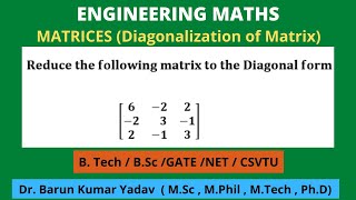
For the matrix A = [4 1; 2 3], the eigenvalues are found to be λ = 5 and λ = 2, and corresponding eigenvectors can be calculated.
An example of a non-diagonalizable matrix is A = [2 1; 0 2], which has repeated eigenvalues and insufficient linearly independent eigenvectors.
Memory Aids
Interactive tools to help you remember key concepts
Rhymes
Eigenvalues help you see, how vectors stretch and flee.
Stories
Imagine a magic door: the matrix is the door, and the eigenvector is the key that unlocks it, revealing the diagonal world.
Memory Tools
PEB: P for eigenvectors, E for eigenvalues, and B for balanced equations.
Acronyms
DIME
Diagonalization
Invertibility
Multiplicity
Eigenvalues.
Flash Cards
Glossary
- Diagonal Matrix
A matrix where all entries outside the main diagonal are zero.
- Eigenvalue
A scalar λ such that for a matrix A and a non-zero vector v, Av = λv.
- Eigenvector
A non-zero vector that changes at most by a scalar factor during the application of a linear transformation.
- Characteristic Polynomial
A polynomial obtained by calculating det(A - λI), used to find eigenvalues.
- Invertible Matrix
A square matrix that has an inverse, meaning there exists another matrix that, when multiplied together, yields the identity matrix.
Reference links
Supplementary resources to enhance your learning experience.