
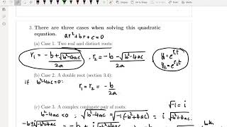
Case III: Complex Roots
Enroll to start learning
You’ve not yet enrolled in this course. Please enroll for free to listen to audio lessons, classroom podcasts and take practice test.
Interactive Audio Lesson
Listen to a student-teacher conversation explaining the topic in a relatable way.
Introduction to Complex Roots
🔒 Unlock Audio Lesson
Sign up and enroll to listen to this audio lesson

Welcome, everyone! Today we will discuss complex roots in differential equations. Can anyone tell me what they think complex roots imply in this context?

I think they represent solutions that involve oscillations, right?
Exactly! Complex roots arise from the auxiliary equation, and they indicate oscillatory solutions. We denote them as m = α ± iβ. Does anyone know how we formulate the general solution from these roots?

Is it something like y(x) = e^(αx)(C₁ cos(βx) + C₂ sin(βx))?
Correct! Good job! This expression shows that the solution has both exponential growth or decay from e^(αx) and the oscillatory behavior from the cosine and sine functions.
To remember this, think of the acronym 'ECO' — Exponential parts COntribute to growth/decay while oscillatory parts are due to sine and cosine. Let’s ensure we understand that structure!

How do we use these in real life?
Great question! These solutions are used in engineering for modeling damped vibrations, as we might encounter in structures subject to dynamic loads.
Let's summarize: Complex roots lead to a general solution of y(x) = e^(αx)(C₁ cos(βx) + C₂ sin(βx)). This includes oscillatory motion and exponential behavior.
Applications of Complex Roots
🔒 Unlock Audio Lesson
Sign up and enroll to listen to this audio lesson

Can anyone think of an application where complex roots are applicable in civil engineering?

Maybe in modeling damped vibrations in buildings?
Precisely! Such models help us assess how structures react to vibrations caused by factors like wind or earthquakes. Why is it essential to understand these vibrations?
To prevent structural failure and ensure safety!
Exactly! Understanding the oscillatory solutions allows us to design structures that can withstand dynamic forces effectively. So, what’s the general solution again?
y(x) = e^(αx)(C₁ cos(βx) + C₂ sin(βx))
Well done! Let's recap: Complex roots are instrumental in engineering because they model oscillatory behaviors critical for safety and design.
Solving Differential Equations with Complex Roots
🔒 Unlock Audio Lesson
Sign up and enroll to listen to this audio lesson
Let's tackle an example: Suppose we have the auxiliary equation m² + 4 = 0. What does this tell us about the roots?
The roots will be complex since the solution to that is m = ±2i.
Right! So what would our general solution look like?
It would be y(x) = e^(0)(C cos(2x) + C sin(2x)). Since α is 0, it simplifies to C₁ cos(2x) + C₂ sin(2x).
Excellent! Remember that if α is zero, we simply observe oscillatory behavior. Now, if we relate this back to vibrations in buildings, what can we infer?
The structure would experience purely periodic motion without any growth or decay.
Yes, precisely! Let’s encapsulate today’s topics: Complex roots lead to oscillatory solutions applicable in various scenarios, including structural dynamics.
Understanding Constants in the Solutions
🔒 Unlock Audio Lesson
Sign up and enroll to listen to this audio lesson
So, we have our general solution involving constants C₁ and C₂. What role do these constants play?
They are determined by the initial or boundary conditions specified for the problem.
Great point! If we modify the conditions, will the solution react accordingly?
Yes! Different conditions will produce different constants leading to various oscillatory behaviors in the solution.
Exactly! So, how about a recap: What do we know about complex roots and their role in engineering?
Complex roots model oscillatory motion, and the constants depend on specific conditions!
Fantastic! You’ve all grasped a fundamental application of complex roots in differential equations.
Introduction & Overview
Read summaries of the section's main ideas at different levels of detail.
Quick Overview
Standard
In this section, we explore the case of complex roots in second-order linear homogeneous differential equations. When the roots of the auxiliary equation are complex conjugates, the general solution reflects oscillatory motion, which is particularly useful in modeling situations such as damped vibrations. The solution is expressed in terms of exponential and trigonometric functions.
Detailed
Detailed Summary
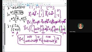
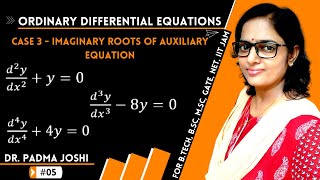
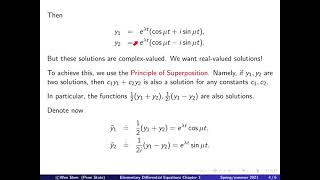
The section discusses Case III of second-order linear homogeneous differential equations characterized by complex roots. When the auxiliary equation results in complex conjugate roots of the form m = α ± iβ, the general solution can be formulated as:
y(x) = e^(αx)(C₁ cos(βx) + C₂ sin(βx))
In this representation, 'C₁' and 'C₂' are constants determined by specific initial or boundary conditions. This form of the solution is crucial in engineering applications, particularly in modeling oscillatory behavior and damped vibrations. The oscillatory components (cos and sin) signify physical systems' responses that exhibit periodic motion, making this understanding vital in fields like civil engineering, where structures may experience oscillations under dynamic loads, such as earthquakes.
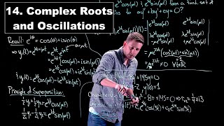
Youtube Videos


Audio Book
Dive deep into the subject with an immersive audiobook experience.
Introduction to Complex Roots
Chapter 1 of 3
🔒 Unlock Audio Chapter
Sign up and enroll to access the full audio experience
Chapter Content
If the roots are complex conjugates:
m=α±iβ
Detailed Explanation
In this case, the roots of the characteristic equation are not real numbers but complex numbers. Complex roots occur in pairs, known as complex conjugates, which can be expressed in the form α ± iβ, where α is the real part and β is the imaginary part. This signifies that the system has oscillatory behavior.
Examples & Analogies
Think of complex roots like the combined motion of a pendulum swinging back and forth while progressively losing height. The pendulum represents the system's oscillation, with the real part showing how it stabilizes over time, while the imaginary part reflects the cyclical nature of the swing.
General Solution for Complex Roots
Chapter 2 of 3
🔒 Unlock Audio Chapter
Sign up and enroll to access the full audio experience
Chapter Content
Then the general solution becomes:
y(x)=eαx (C cosβ x+C sinβx)
Detailed Explanation
The general solution for a second-order differential equation with complex roots combines exponential decay or growth with sine and cosine functions. The term e^(αx) represents the exponential change dictated by the real part of the roots, while C cos(βx) and C sin(βx) account for the oscillatory behavior introduced by the imaginary part. Here, C is a constant that can vary based on initial conditions.
Examples & Analogies
Imagine you are pushing a child on a swing. As you push (the exponential term), the swing moves higher (exponential growth) while also swinging back and forth (oscillatory motion). The swings represent the sine and cosine functions, showing how the system moves in a periodic manner.
Application in Engineering
Chapter 3 of 3
🔒 Unlock Audio Chapter
Sign up and enroll to access the full audio experience
Chapter Content
This form is particularly useful in modeling damped vibrations or oscillatory motion.
Detailed Explanation
In engineering, the solution found with complex roots is crucial for analyzing systems that experience damped vibrations, such as beams subjected to dynamic loading. The use of cos and sin indicates that the system will oscillate but might lose energy over time due to damping, which is represented by α in the exponential term.
Examples & Analogies
Consider a car's suspension system as it travels over a bumpy road. The car oscillates (up and down) in response to bumps but eventually stabilizes. This stabilization can be modeled using the general solution involving complex roots, giving engineers a way to predict how the car's suspension will behave over time.
Key Concepts
-
Complex Roots: Indicate periodic solutions in differential equations.
-
Homogeneous Equation: Solutions revolve around the form of the related polynomial characteristic equation.
-
Auxiliary Equation: A tool to find potential solutions to differential equations.
Examples & Applications
If the auxiliary equation is m^2 + 4 = 0, the roots would be ±2i, leading to the general solution y(x) = C₁ cos(2x) + C₂ sin(2x).
Damped vibrations in a structure can be modeled by y(x) = e^(−bx)(C₁ cos(ωx) + C₂ sin(ωx)), where 'b' causes exponential decay.
Memory Aids
Interactive tools to help you remember key concepts
Rhymes
Complex roots show what we need, Oscillations are their creed.
Stories
Imagine a bridge swaying gently in the wind; it oscillates back and forth, not collapsing but moving steadily—this is akin to solutions with complex roots.
Memory Tools
COSINE creates Oscillations, SINE shows oscillatory NEtworks — COS + SINE together signify complex roots' behavior.
Acronyms
ECO
Exponential decay and oscillations create solutions.
Flash Cards
Glossary
- Complex Roots
Roots of a polynomial that are not real, expressed in the form of a ± bi, where a and b are real numbers.
- Homogeneous Differential Equation
A differential equation is homogeneous if it can be written in the form where all terms are a function of the dependent variable and its derivatives.
- Auxiliary Equation
An algebraic equation derived from a differential equation, used to find the characteristic roots.
- Oscillatory Motion
Motion that repeatedly fluctuates or oscillates, often between two points.
- Exponential Behavior
The behavior of a function that grows or decays at a rate proportional to its current value.
Reference links
Supplementary resources to enhance your learning experience.