
Homogeneous Linear Equations of Second Order
Enroll to start learning
You’ve not yet enrolled in this course. Please enroll for free to listen to audio lessons, classroom podcasts and take practice test.
Interactive Audio Lesson
Listen to a student-teacher conversation explaining the topic in a relatable way.
Introduction to Homogeneous Linear Equations
🔒 Unlock Audio Lesson
Sign up and enroll to listen to this audio lesson

Today, we will delve into homogeneous linear equations of the second order, essential in civil engineering. Can anyone tell me what a second-order differential equation looks like?

Isn't it something like d²y/dx² + b dy/dx + c y = 0?
Exactly! This form helps describe various physical phenomena. Now, who can tell me the significance of the coefficient functions a(x), b(x), and c(x)?

They determine the behavior of the system being modeled, right?
Correct! Remember, a(x) must be non-zero. Let’s explore the consequences of having constant coefficients.
Cases of Roots and General Solutions
🔒 Unlock Audio Lesson
Sign up and enroll to listen to this audio lesson

Now let's discuss the types of roots we can encounter. What happens when the auxiliary equation has distinct real roots?

Oh, that’s when we have two different roots, right? The general solution would be the sum of two exponentials!
Precisely! The solution takes the form $y(x) = C_1 e^{m_1 x} + C_2 e^{m_2 x}$. What about when we have repeated roots?

In that case, it would be $y(x) = (C_1 + C_2 x)e^{m x}$, which accounts for the repeated root.
Great job! Lastly, how do we handle complex roots?
With complex roots, the solution has a sine and cosine component, right?
Yes! It's $y(x) = e^{\alpha x} (C_1 \cos(\beta x) + C_2 \sin(\beta x))$. This is crucial in modeling oscillation.
Application Examples in Engineering
🔒 Unlock Audio Lesson
Sign up and enroll to listen to this audio lesson
Let’s apply our knowledge! How would the solutions to these equations manifest in real-world engineering scenarios?
We can see them in beam deflections under dynamic loading situations.
Absolutely! These equations help us analyze structural integrity. Any thoughts on thermal analysis?
Temperature distribution would lead to similar second-order equations, guiding heat transfer design.
Excellent insights! Remember, these methods are fundamental to ensuring safety and reliability in engineering designs.
Numerical Methods and Limitations
🔒 Unlock Audio Lesson
Sign up and enroll to listen to this audio lesson
What happens when we can't find an exact solution?
We might have to use numerical methods!
Exactly! Techniques like Euler’s method and the Runge-Kutta can be invaluable. Does anyone know why these methods are crucial?
They help solve equations that are too complex for analytical solutions, right?
Exactly! Real-world applications are often non-linear or have varying conditions. Let’s reinforce why understanding these methods is important for our future careers.
Review and Reinforcement
🔒 Unlock Audio Lesson
Sign up and enroll to listen to this audio lesson
Let’s summarize what we've learned. What are the solutions based on the type of roots?
Distinct roots yield different exponentials, repeated roots yield a linear term multiplied by an exponential, and complex roots introduce oscillatory terms.
Perfect! And in which applications might we utilize these equations?
Vibrations of beams, thermal analysis, and structural mechanics!
Fantastic! Remember, these concepts are foundational to understanding more complex systems in civil engineering.
Introduction & Overview
Read summaries of the section's main ideas at different levels of detail.
Quick Overview
Standard
The section provides an overview of homogeneous linear second-order differential equations, including their definition, methods of solving them through various cases (distinct real roots, repeated roots, and complex roots), and applications in engineering fields, such as vibrations in beams and thermal analysis.
Detailed
Homogeneous Linear Equations of Second Order
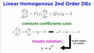
This section explores the definition and significance of homogeneous linear second-order differential equations in civil engineering, emphasizing their role in modeling mechanical vibrations, heat conduction, fluid flow, and elasticity. The general form of a second-order linear homogeneous differential equation is defined as:
$$\frac{d^2y}{dx^2} + b(x)\frac{dy}{dx} + c(x)y = 0$$
where $y = y(x)$ is the unknown function, and $a(x)$, $b(x)$, and $c(x)$ are functions of the independent variable $x$ with $a(x) \neq 0$. The section then discusses the particular case of constant coefficients, which is pivotal in engineering applications.
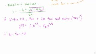
The key solution methods involve the auxiliary (characteristic) equation derived from an assumed solution of the form $y = e^{mx}$. The nature of the roots of this equation determines the solution’s form:
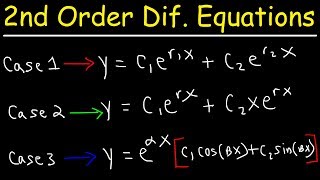
- Case I: Real and Distinct Roots
When the auxiliary equation has two distinct real roots, the general solution is of the form $y(x) = C_1 e^{m_1 x} + C_2 e^{m_2 x}$. - Case II: Real and Repeated Roots
If both roots are equal, the solution takes the form $y(x) = (C_1 + C_2 x)e^{m x}$. - Case III: Complex Roots
For complex conjugate roots, the solution becomes $y(x) = e^{\alpha x} (C_1 \cos(\beta x) + C_2 \sin(\beta x))$.
Finally, practical examples illustrate each case, demonstrating how these differential equations apply to scenarios such as beam vibrations, thermal analysis, and structural mechanics, underscoring their significance in real-world engineering contexts.
Youtube Videos

Audio Book
Dive deep into the subject with an immersive audiobook experience.
Definition of Second-Order Linear Homogeneous Equation
Chapter 1 of 4
🔒 Unlock Audio Chapter
Sign up and enroll to access the full audio experience
Chapter Content
A second-order linear homogeneous differential equation has the general form:
d²y
dy
a(x) + b(x) + c(x)y = 0
dx²
dx
Where:
- y = y(x) is the unknown function of the independent variable x
- a(x), b(x), c(x) are given functions of x
- a(x) ≠ 0
If a(x), b(x), c(x) are constants, the equation is said to have constant coefficients.
Detailed Explanation
In mathematics, a second-order linear homogeneous differential equation is used to describe various physical phenomena. The equation consists of a function, its derivatives, and coefficients that might depend on the variable. Here, 'second-order' means it involves the second derivative of the function, 'linear' indicates that the function and its derivatives appear to the first power, and 'homogeneous' means there are no additional functions added that depend on the variable. If the coefficients (a, b, c) are constant values, it simplifies the equation significantly and makes it easier to solve.
Examples & Analogies
Think of this equation like a recipe. The coefficients (a, b, c) are like the specific amounts of ingredients required to bake a cake (the unknown function y). Just as you cannot bake a cake properly without following the recipe (the equation), many physical systems cannot be accurately modeled without these differential equations.
Homogeneous Linear Equations with Constant Coefficients
Chapter 2 of 4
🔒 Unlock Audio Chapter
Sign up and enroll to access the full audio experience
Chapter Content
The most common and solvable form in engineering applications is:
d²y
dy
a + b + c y = 0
dx²
dx
Dividing through by a (assuming a ≠ 0):
d²y
dy
+p + qy = 0
dx²
dx
Where:
- p = b/a
- q = c/a
Detailed Explanation
This portion focuses on a specific version of the second-order linear homogeneous differential equation where the coefficients are constant. By dividing through by 'a,' we transform the equation into a simpler form, which often makes it easier to work with. The parameters 'p' and 'q' represent normalized forms of the coefficients 'b' and 'c,' providing a clearer path for solving the equation. Engineers typically encounter this form because it applies to many practical problems, such as vibrations in structures.
Examples & Analogies
Imagine adjusting the volume of music on a sound system. The coefficients represent different factors affecting the sound (like bass, treble, etc.). By normalizing those factors (like adjusting everything to a baseline level), you can better appreciate the overall quality of the sound, much like simplifying the equation allows us to focus on its core aspects.
Auxiliary Equation and General Solution
Chapter 3 of 4
🔒 Unlock Audio Chapter
Sign up and enroll to access the full audio experience
Chapter Content
To solve:
d²y
dy
+p + qy = 0
dx²
dx
We assume a solution of the form:
y = e^(mx)
Substituting into the differential equation:
m²e^(mx) + pm e^(mx) + qe^(mx) = 0
e^(mx) (m² + pm + q) = 0
Since e^(mx) ≠ 0,
the auxiliary equation (characteristic equation) is:
m² + pm + q = 0
The nature of the roots of the auxiliary equation determines the form of the general solution.
Detailed Explanation
To find solutions to the homogeneous equation, we assume a solution of a specific exponential form, 'e^(mx)'. When we substitute this into the equation and simplify, we derive what is known as the auxiliary or characteristic equation. The roots of this equation tell us critical information about the solution's behavior. Specifically, they determine whether the solutions will be real, complex, or repeated, which directly affects the shape and characteristics of the solution curves we will derive.
Examples & Analogies
Think of trying to determine the path of a thrown ball. Finding the right formula to describe its motion (the differential equation) is like solving for a point in the air (the equation). The type of trajectory (the form of the general solution) depends on how hard or at what angle you throw it (the roots of the auxiliary equation).
Cases of Roots and General Solutions
Chapter 4 of 4
🔒 Unlock Audio Chapter
Sign up and enroll to access the full audio experience
Chapter Content
-
Case I: Real and Distinct Roots
If the auxiliary equation has two distinct real roots m₁ and m₂, then:
y(x) = C₁ e^(m₁x) + C₂ e^(m₂x)
Where C₁ and C₂ are arbitrary constants determined by initial/boundary conditions. -
Case II: Real and Repeated Roots
If the roots are real and equal, say m₁ = m₂ = m, then:
y(x) = (C₁ + C₂ x) e^(mx)
This accounts for the multiplicity of the solution space. -
Case III: Complex Roots
If the roots are complex conjugates:
m = α ± iβ
Then the general solution becomes:
y(x) = e^(αx) (C₁ cos(βx) + C₂ sin(βx))
This form is particularly useful in modeling damped vibrations or oscillatory motion.
Detailed Explanation
The roots of the auxiliary equation reveal different scenarios for general solutions. If both roots are distinct and real, the solution is a combination of two exponential functions. If the roots are real and repeated, we introduce a linear term because the function has less 'freedom' due to the repeated root. Lastly, if the roots are complex, we can use trigonometric functions to describe oscillatory behavior, as complex roots indicate that the system is likely to exhibit wave-like properties. Each case highlights different physical behaviors observed in real-life applications.
Examples & Analogies
Consider a swing in a park. When someone pushes it gently (distinct roots), it swings smoothly. If two people push it at the same time but with equal strength (repeated roots), it may not swing as much but stays in place (a linear modification). Lastly, when a strong gust of wind causes it to sway back and forth (complex roots), it creates an undulating pattern that resembles oscillations common in physical systems.
Key Concepts
-
Homogeneous Linear Equation: Defined as an equation that can be expressed as a linear combination of its derivatives.
-
Auxiliary Equation: A key step in solving differential equations, derived from assuming a solution of a specific form.
-
Distinct Roots: Real and different roots lead to individual exponential solutions that are summed.
-
Repeated Roots: Identical roots necessitate a linear term to be added to the exponential solution.
-
Complex Roots: Present sine and cosine components in the solution, often modeling periodic behavior.
Examples & Applications
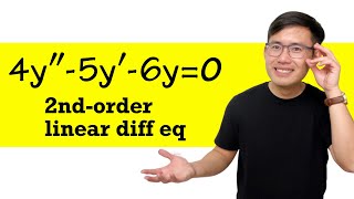
Example 1: Solve the equation \(\frac{d^2y}{dx^2} - 5 \frac{dy}{dx} + 6y = 0\): Roots m=2,3 and solution \(y(x) = Ce^{2x} + Ce^{3x}\).
Example 2: Solve \(\frac{d^2y}{dx^2} - 4 \frac{dy}{dx} + 4y = 0\): Repeated root m=2 and solution \(y(x) = (C_1 + C_2 x)e^{2x}\).
Example 3: Solve \(\frac{d^2y}{dx^2} + 4y = 0\): Complex roots \(m = ±2i\) and solution \(y(x) = C \cos(2x) + C \sin(2x)\).
Memory Aids
Interactive tools to help you remember key concepts
Rhymes
For beams that shake and structures sway, homogeneous roots help find the way!
Stories
Imagine a bridge vibrating in a storm. Homogeneous equations help engineers calm the storm through precise calculations.
Memory Tools
R.E.C. - Remember Each Case: Real Distinct, Repeated, Complex.
Acronyms
HLSO - Homogeneous Linear Second Order.
Flash Cards
Glossary
- Homogeneous Linear Differential Equation
An equation of the form \(a(x) \frac{d^2y}{dx^2} + b(x) \frac{dy}{dx} + c(x)y = 0\) where the functions are linear and homogeneous.
- Auxiliary Equation
The characteristic equation obtained from assuming a solution of the form \(y = e^{mx}\), leading to the equation \(m^2 + pm + q = 0\).
- Distinct Roots
Two different real roots of the auxiliary equation, leading to a solution with two exponential functions.
- Repeated Roots
Two equal roots of the auxiliary equation, resulting in a solution composed of a linear term multiplied by an exponential.
- Complex Roots
Roots of the auxiliary equation that are not real numbers, resulting in trigonometric components in the general solution.
Reference links
Supplementary resources to enhance your learning experience.