
Homogeneous Linear Equations with Constant Coefficients
Enroll to start learning
You’ve not yet enrolled in this course. Please enroll for free to listen to audio lessons, classroom podcasts and take practice test.
Interactive Audio Lesson
Listen to a student-teacher conversation explaining the topic in a relatable way.
Introduction to Homogeneous Linear Equations
🔒 Unlock Audio Lesson
Sign up and enroll to listen to this audio lesson

Today, we're diving into homogeneous linear equations with constant coefficients, which are pivotal in many engineering scenarios. Who can tell me what a differential equation is?

I think it’s an equation involving derivatives?
Exactly! Specifically, we're focusing on second-order differential equations. Can someone tell me what 'homogeneous' means in this context?

Does it mean there are no constant terms, like the equation equals zero?
Right! Now, let's move to the general form: \( \frac{d^2y}{dx^2} + p \frac{dy}{dx} + qy = 0 \). Here, \( p \) and \( q \) are constants. Remember this form—let's use a mnemonic: 'Pursue Quality' for p and q!
Understanding the Auxiliary Equation
🔒 Unlock Audio Lesson
Sign up and enroll to listen to this audio lesson

Now, let's discuss solving the equation. We assume a solution \( y = e^{mx} \). What happens when we substitute that into our equation?

We get the auxiliary equation: \( m^2 + pm + q = 0 \)!
Correct! This is also known as the characteristic equation. Can anyone explain how the roots of this equation affect our solution?

If we have distinct roots, the general solution is different than if we have repeated or complex roots!
Yes! Let's remember this with the acronym R.D.C.: Real Distinct, Real Repeated, Complex.
Case Distinctions Based on Roots
🔒 Unlock Audio Lesson
Sign up and enroll to listen to this audio lesson
Let's break down the solution forms! When we have distinct real roots, how does our solution look?
It looks like \( y(x) = C_1 e^{m_1 x} + C_2 e^{m_2 x} \)!
Good! And for repeated roots, what changes?
The solution becomes: \( y(x) = (C_1 + C_2 x)e^{mx} \)!
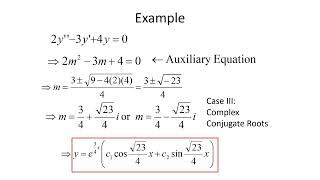
Exactly! Lastly, what if we have complex roots?
It would take the form: \( y(x) = e^{\alpha x} (C_1 \cos(\beta x) + C_2 \sin(\beta x)) \)!
Great job! Remember to visualize how each of these solutions would behave graphically.
Real-World Applications
🔒 Unlock Audio Lesson
Sign up and enroll to listen to this audio lesson
Now let’s connect these concepts to civil engineering! Can someone describe how these equations show up in our field?
In analyzing the vibrations of beams or columns!
Correct! For example, the deflection of beams can be modeled as a second-order equation. Why is this relevant in the design of structures?
Because we need to ensure they can withstand loads safely!
Absolutely! Remember, understanding these concepts allows us to predict structural behaviors effectively.
Introduction & Overview
Read summaries of the section's main ideas at different levels of detail.
Quick Overview
Standard
The section discusses the structure of homogeneous linear equations with constant coefficients, leading to the derivation of the auxiliary equation. It categorizes the general solution based on the nature of the roots and provides context on their relevance in civil engineering applications through examples.
Detailed
Homogeneous Linear Equations with Constant Coefficients
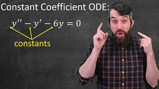
In civil engineering, second-order homogeneous linear differential equations with constant coefficients play a critical role in analyzing structures under various conditions. The general form of such equations is given as:
$$\frac{d^2y}{dx^2} + p \frac{dy}{dx} + qy = 0$$
where \( p \) and \( q \) are constants derived from the coefficients of the original differential equation. To solve these equations, we assume a solution of the form \( y = e^{mx} \), leading to the characteristic (auxiliary) equation:
$$m^2 + pm + q = 0$$
The nature of the roots (real distinct, real repeated, or complex) subsequently determines the specific form of the general solution. This section also highlights the importance of these equations in engineering applications, demonstrating through numerous examples that range from solving differential equations to understanding mechanical vibrations, thermal analysis, and structural mechanics.
Youtube Videos


Audio Book
Dive deep into the subject with an immersive audiobook experience.
General Form of Homogeneous Linear Equations
Chapter 1 of 2
🔒 Unlock Audio Chapter
Sign up and enroll to access the full audio experience
Chapter Content
The most common and solvable form in engineering applications is:
d²y
dy
a + b + c y = 0
dx²
dx
Detailed Explanation
This chunk introduces the standard form of a second-order homogeneous linear differential equation that typically arises in engineering applications. The equation is expressed with coefficients a, b, and c, which may vary. It is key to note that this structure allows engineers to address various dynamic systems such as vibrations and heat conduction, providing a foundation for deriving solutions in practical scenarios.
Examples & Analogies
Think of this equation as the blueprint for a building. Just as the blueprint outlines the different elements that construct the building, here the coefficients represent different forces working within a system, like gravity or tension. Just as changing a load in the building's blueprint affects its stability, altering these coefficients influences the system's behavior.
Standard Form Adjustment
Chapter 2 of 2
🔒 Unlock Audio Chapter
Sign up and enroll to access the full audio experience
Chapter Content
Dividing through by a (assuming a ≠ 0):
d²y
dy
+p + qy = 0
dx²
dx
Where:
b
• p= ,
a
c
• q= a
Detailed Explanation
In this chunk, we adjust the standard form of the equation by dividing every term by 'a', which normalizes the equation. This reformation is crucial as it converts the equation into a form that allows easier manipulation and solution, dividing into parameters p and q that simplify the analysis. These parameters provide a clearer insight into the behavior of the solutions based on their values.
Examples & Analogies
Imagine modifying a recipe where you adjust the ingredients to standardize proportions for easier cooking. By dividing everything by 'a,' we ensure that the equation is properly scaled, making it more manageable for problem-solving, just as a standardized recipe ensures consistent results.
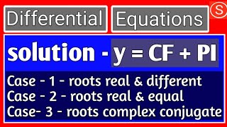
Key Concepts
-
Auxiliary Equation: A characteristic equation formed to find the roots that will determine the general solution.
-
Roots' Nature: Distinct, repeated, and complex roots lead to different general solution forms.
-
Application: Homogeneous linear equations are vital in modeling physical phenomena in civil engineering.
Examples & Applications
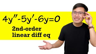
Example 1: If the equation is \(\frac{d^2y}{dx^2} - 5\frac{dy}{dx} + 6y = 0\), then finding the auxiliary equation leads to roots \(m_1=2\) and \(m_2=3\). The general solution will be \(y(x) = C_1 e^{2x} + C_2 e^{3x}\).
Example 2: For a repeated root scenario with \(\frac{d^2y}{dx^2} - 4\frac{dy}{dx} + 4y = 0\), the auxiliary equation gives a root \(m=2\), leading to the solution \(y(x) = (C_1 + C_2x)e^{2x}\.
Example 3: For an equation with complex roots such as \(\frac{d^2y}{dx^2} + 4y = 0\), the roots are \(m=±2i\). The solution takes the form \(y(x)=e^{0x}(C_1 \cos(2x) + C_2 \sin(2x))\).
Memory Aids
Interactive tools to help you remember key concepts
Rhymes
Homogeneous and linear, with roots to discern, / Solutions come from forms, over which we must learn.
Stories
In a land of equations, two roots were tied to a tree of solutions. When they met, they would either grow apart, showing exponential growth, or stay together, leading to shared outcomes, traveling together through oscillations.
Memory Tools
R.D.C. - Remember this to recall: Real Distinct, Real Repeated, Complex roots—each tell a different story.
Acronyms
Pursue Quality
for coefficients p (pressure) and q (quantity) which steer our differential outcomes!
Flash Cards
Glossary
- Homogeneous Linear Equation
An equation where all the terms are linear and there are no constant or non-homogeneous parts.
- Constant Coefficients
Coefficients that do not change with the variable, making the differential equation simpler to solve.
- Auxiliary Equation
The characteristic equation derived from substituting a presumed solution form into a differential equation.
- Roots
Solutions to the auxiliary equation that influence the form of the general solution.
- General Solution
The complete solution of a differential equation, incorporating all possible solutions based on the nature of the roots.
Reference links
Supplementary resources to enhance your learning experience.