
Numerical Solutions of Ordinary Differential Equations
Enroll to start learning
You’ve not yet enrolled in this course. Please enroll for free to listen to audio lessons, classroom podcasts and take practice test.
Interactive Audio Lesson
Listen to a student-teacher conversation explaining the topic in a relatable way.
Introduction to ODEs
🔒 Unlock Audio Lesson
Sign up and enroll to listen to this audio lesson

Let's start by discussing ordinary differential equations, or ODEs. Who can tell me what they are?

ODEs are equations that involve functions and their derivatives with respect to one variable.
Exactly! ODEs are crucial in modeling many real-world phenomena. Can anyone give me an example of where we would use them?

They can be used in population dynamics or physics, right?
Great examples! Now, when we can't find a solution analytically, what do we need to use?

Numerical methods, like Euler's method!
Exactly! Let's explore how numerical methods help us solve ODEs when analytical solutions are complex or impossible.
Euler's Method
🔒 Unlock Audio Lesson
Sign up and enroll to listen to this audio lesson

Now, let's focus on Euler's Method. Who remembers the formula for this method?

The formula is $y_{n+1} = y_n + h imes f(t_n, y_n)$!
Perfect! Can someone explain what the term 'h' signifies?
It represents the step size, the distance between the points.
Correct! This method is known for being simple but has its disadvantages. Can anyone name a disadvantage?
It's low accuracy and can struggle with stiff equations.
Very good observation! Remember, we implement Euler's Method iteratively using previous values to compute the next estimate.
Runge-Kutta Methods
🔒 Unlock Audio Lesson
Sign up and enroll to listen to this audio lesson
Next up is the Runge-Kutta methods. What do we call the most common one?
The fourth-order Runge-Kutta method, or RK4.
That's right! Can someone explain how RK4 improves upon Euler's Method?
It calculates multiple slopes to get a weighted average, making it more accurate.
Exactly! By computing the slopes $k_1, k_2, k_3, k_4$, we achieve better accuracy. How many function evaluations does RK4 require per step?
Four evaluations, which makes it more computationally intense!
Great job! It's indeed more computationally expensive but yields much better results.
Multistep Methods
🔒 Unlock Audio Lesson
Sign up and enroll to listen to this audio lesson
Let's now look at multistep methods. Does anyone know how these differ from single-step methods?
They use multiple previous points instead of just the last one.
Exactly! For instance, the Adams-Bashforth method is a type of explicit multistep method. Can you recall its formula?
It's $y_{n+1} = y_n + \frac{h}{2} [3f(t_n, y_n) - f(t_{n-1}, y_{n-1})]$.
Spot on! And what are some advantages of using the Adams-Bashforth methods?
They're generally more accurate for the same number of function evaluations!
Absolutely! However, they do have a downside. What is it?
They require several previous function values, which may not always be available.
Correct! Remember that the choice of method depends on the characteristics of the ODE we’re trying to solve.
Comparison of Methods
🔒 Unlock Audio Lesson
Sign up and enroll to listen to this audio lesson
Let’s summarize what we've learned about the various numerical methods. Can someone list the methods we’ve discussed?
We’ve talked about Euler's method, Runge-Kutta methods, and Multistep methods.
Correct! Now, how would you compare their computational costs and accuracy?
Euler's Method is the least accurate and easiest, while RK4 is more accurate but computationally expensive.
And Multistep methods can be very efficient but rely on past data.
Exactly! Each method has trade-offs between accuracy, stability, and computational effort. Always consider the problem’s nature when choosing a method.
Introduction & Overview
Read summaries of the section's main ideas at different levels of detail.
Quick Overview
Standard
This section introduces ordinary differential equations (ODEs) and their significance in various fields. It explores numerical methods, specifically Euler's Method, Runge-Kutta Methods, and Multistep Methods, detailing their processes, advantages, disadvantages, and applications.
Detailed
Detailed Summary
Ordinary differential equations (ODEs) are equations that involve functions of a single variable and their derivatives, important for modeling various real-world phenomena. When analytical solutions are not feasible, numerical methods become necessary. This chapter covers three primary methods:
Euler's Method
Euler’s Method is a straightforward technique that approximates ODE solutions by discretizing the time domain into small steps and iteratively updating the solution. The formula is given by:
$$y_{n+1} = y_n + h imes f(t_n, y_n)$$
Where $h$ is the step size. Despite its simplicity, it has low accuracy and can be unstable for stiff equations.
Example: For the ODE $\frac{dy}{dt} = y, y(0) = 1$ with $h=0.1$, the method produces successive approximations based on the previous value.
Runge-Kutta Methods
The Runge-Kutta methods, especially the fourth-order method (RK4), provide improved accuracy. They compute four intermediate slopes to form a better estimate:
$$y_{n+1} = y_n + \frac{1}{6}(k_1 + 2k_2 + 2k_3 + k_4)$$
Where each $k$ represents the slopes calculated at various stages. RK4 is more accurate than Euler's method but computationally more expensive.
Multistep Methods
Multistep methods utilize information from multiple previous steps to better estimate the solution. For example, the Adams-Bashforth method uses previous values for better approximation while the Adams-Moulton method is implicit and tends to be more stable, especially for stiff equations.
Comparison of Methods
Finally, a comparison highlights the trade-offs: Euler's method is easy but inaccurate; RK4 is accurate but expensive; and Multistep methods, while efficient, require more past data. Overall, the choice of method depends on the ODE’s characteristics and the computational resources available.
Youtube Videos

Audio Book
Dive deep into the subject with an immersive audiobook experience.
Introduction to Ordinary Differential Equations (ODEs)
Chapter 1 of 6
🔒 Unlock Audio Chapter
Sign up and enroll to access the full audio experience
Chapter Content
An ordinary differential equation (ODE) is an equation involving functions of a single variable and their derivatives. ODEs are fundamental in modeling various real-world phenomena, such as physical systems, population dynamics, and chemical reactions. The initial value problem (IVP) for an ODE requires finding a solution to the equation given an initial condition, i.e., the value of the function at a particular point.
Numerical methods are essential for solving ODEs when exact analytical solutions are difficult or impossible to obtain. This chapter covers the most commonly used numerical methods for solving ODEs: Euler’s method, Runge-Kutta methods, and Multistep methods.
Detailed Explanation
An ordinary differential equation (ODE) involves functions of a single variable and their derivatives. For example, a common situation might be determining how a population changes over time, which can be modeled with ODEs. The initial value problem (IVP) means we need to find the function given its value at a specific starting point. When analytical solutions are hard to find—due to complexity or intractability—numerical methods come into play. This chapter aims to introduce popular numerical methods for ODEs, including Euler’s method, Runge-Kutta methods, and Multistep methods, which offer practical solutions to get approximations of ODEs.
Examples & Analogies
Imagine you're trying to predict the growth of a tree over time. You know the tree's height today (the initial condition), but you don’t have a formula to calculate its height every day. By using numerical methods like those introduced in this chapter, you can estimate the tree’s height on future days based on its current growth rate.
Euler's Method
Chapter 2 of 6
🔒 Unlock Audio Chapter
Sign up and enroll to access the full audio experience
Chapter Content
Euler’s method is one of the simplest and most straightforward numerical techniques for solving ODEs. It approximates the solution of the ODE by discretizing the time domain into small steps and iteratively updating the solution based on the function's derivative.
Detailed Explanation
Euler's method is a basic approach to approximating solutions for ordinary differential equations. The key idea is to break the problem into small time increments or steps and update the solution iteratively using the derivative at the current point. Each step involves calculating the next value based on the current value and the slope derived from the ODE. This approach is intuitive and easy to implement, making it an essential starting point for learning numerical methods.
Examples & Analogies
Consider a car moving down a straight road. If you want to estimate how far it will go in the next few seconds, you take the current speed (the derivative) and multiply it by the time increment. Just like using Euler's method, you can keep updating the estimated distance at small intervals to see how far the car travels over time.
The Euler Method Formula
Chapter 3 of 6
🔒 Unlock Audio Chapter
Sign up and enroll to access the full audio experience
Chapter Content
Given an ODE of the form:
dydt=f(t,y),y(t0)=y0
Euler’s method approximates the solution at each step as:
yn+1=yn+h⋅f(tn,yn)
Where:
● yny_n is the approximation of the solution at step nn,
● hh is the step size (the distance between successive points),
● f(tn,yn)f(t_n, y_n) is the derivative of yy at the point (tn,yn)(t_n, y_n).
Detailed Explanation
The Euler method formula provides a systematic way to compute successive approximations of the solution to an ODE. You start with a known point (e.g., the initial condition). The equation gives you a way to find the next value (yn+1) by taking the current value (yn) and adding the product of the step size (h) and the derivative (f(tn, yn)). Here, 'ty' represents the output of the function at the current point. This formula encapsulates how the method builds up an approximation step by step.
Examples & Analogies
Think of making cupcakes. You start with a certain amount of flour (your initial state). Each time you add more flour based on a recipe, that represents your step size, while the amount needed (function output) changes slightly as you keep adding. Just as you calculate the new total flour incrementally, Euler's formula calculates the next step in solving the ODE.
How Euler’s Method Works
Chapter 4 of 6
🔒 Unlock Audio Chapter
Sign up and enroll to access the full audio experience
Chapter Content
- Start with an initial condition y(t0)=y0.
- Compute the derivative f(t0,y0) using the ODE.
- Use the Euler update formula to compute y1 at the next step.
- Repeat the process for each subsequent step, using the previous solution to calculate the next one.
Detailed Explanation
The steps of Euler's method can be summarized in a straightforward sequence. First, you determine your starting point. Next, you find the derivative at that point. Using the derivative, you apply the formula to find the next value. You then repeat this process iteratively, each time using the latest calculated value to find the next one. This method continues until you reach your desired time frame or point.
Examples & Analogies
Imagine you are walking along a path. You decide to step forward a small distance (step size), but you want to know how steep the path is at each step (your slope or derivative). Every time you check and take another step based on where you are currently, that's similar to using Euler’s method to navigate your way along the route.
Advantages and Disadvantages of Euler’s Method
Chapter 5 of 6
🔒 Unlock Audio Chapter
Sign up and enroll to access the full audio experience
Chapter Content
Advantages:
- Very simple to implement and understand.
- Computationally inexpensive.
Disadvantages:
- Low accuracy: Euler’s method is only a first-order method, meaning the error decreases linearly with the step size h.
- Instability: For stiff equations or large step sizes, Euler’s method may produce inaccurate or unstable results.
Detailed Explanation
Euler's method is appealing because of its simplicity and low computational cost. These features make it accessible for beginners. However, its major drawbacks are low accuracy, especially with larger step sizes, and potential instability when applied to certain types of equations (stiff equations). Being a first-order method means that reducing your step size will lower the error only linearly, which may not be sufficient for precise calculations.
Examples & Analogies
Consider using a basic map app to get directions while driving. While the app can give you an overview (simple to understand), it might not account for complex road conditions or traffic (low accuracy). Similarly, while Euler’s method seems straightforward, it may not suffice for all situations, especially those requiring detailed analysis.
Euler's Method Example
Chapter 6 of 6
🔒 Unlock Audio Chapter
Sign up and enroll to access the full audio experience
Chapter Content
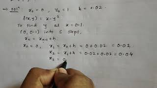
For the ODE:
dydt=y,y(0)=1
Euler's method approximates the solution at each step as follows:
- Let h=0.1 be the step size.
- For t0=0,y0=1:
y1=y0+h⋅f(t0,y0)=1+0.1⋅1=1.1
- Repeat for the next steps, updating yn using the Euler formula.
Detailed Explanation
This example demonstrates the application of Euler's method with a specific ODE. Starting with an initial condition, we choose a small step size (h=0.1) and calculate the next value step-by-step. This gives a concrete understanding of how the theoretical formula is practically applied and how values evolve over time as we continue using the Euler formula.
Examples & Analogies
Think of filling a balloon with air. Each time you add air (the defined step size), you measure the new size of the balloon (the updated function value). In this example, you start with a known size, and with each breath of air (application of the formula), you can see how the balloon grows.
Key Concepts
-
Ordinary Differential Equations (ODEs): Equations involving functions and their derivatives.
-
Euler's Method: A straightforward numerical method for approximating solutions of ODEs.
-
Runge-Kutta Methods (RK4): A more accurate method that uses intermediate slopes for better estimates.
-
Multistep Methods: Techniques that utilize previous points to improve accuracy and efficiency.
Examples & Applications
Using Euler's Method for the ODE dydt=y, y(0)=1 with h=0.1, produces successive approximations, such as y1=1.1.
In applying RK4 for the same equation, we compute k1, k2, k3, k4, resulting in a more accurate value than that from Euler's Method.
Memory Aids
Interactive tools to help you remember key concepts
Rhymes
When Euler wants to guess a new, he looks at the old and sees what's true.
Stories
Imagine a hiker (ODE) navigating a steep hill. With each step (function value), he checks with his guide (derivative) to decide his next step (new approximation). The guide gives him the best advice (accuracy) but requires consistency in direction (correct step size).
Memory Tools
Remember the acronym R-U-M for Runge-Kutta, Euler's, and Multistep Methods in solving ODEs.
Acronyms
Use the acronym E-M-R for Remembering the methods
Euler (E)
Multistep (M)
Runge-Kutta (R).
Flash Cards
Glossary
- Ordinary Differential Equation (ODE)
An equation involving functions of a single variable and their derivatives.
- Initial Value Problem (IVP)
Finding a solution to an ODE given the value of the function at a certain point.
- Euler's Method
A simple first-order numerical method for approximating solutions of ODEs.
- RungeKutta Methods
A group of methods used to solve ODEs, notably the fourth-order method (RK4) which is more accurate.
- Multistep Methods
Methods that use information from multiple previous steps to estimate the next value.
- AdamsBashforth Method
An explicit multistep method that uses multiple past points for ODE approximation.
- AdamsMoulton Method
An implicit multistep method combining current and previous points, known for better stability.
Reference links
Supplementary resources to enhance your learning experience.