
Long Run Costs
Enroll to start learning
You’ve not yet enrolled in this course. Please enroll for free to listen to audio lessons, classroom podcasts and take practice test.
Interactive Audio Lesson
Listen to a student-teacher conversation explaining the topic in a relatable way.
Introduction to Long Run Costs
🔒 Unlock Audio Lesson
Sign up and enroll to listen to this audio lesson

Today, we'll learn about long run costs. In the long run, all inputs are variable, unlike in the short run where some factors are fixed. Can someone explain what that means?

Does that mean that companies can adjust everything they use for production?
Great question! Yes, firms can adjust all inputs, allowing them to optimize production and reduce costs. This flexibility is crucial for adapting to market changes.

So, what is the main difference between total cost and total variable cost in the long run?
In the long run, total cost and total variable cost are the same because there are no fixed costs—meaning all costs are variable.

How do we calculate long run average cost, then?
That's an excellent point! Long run average cost, or LRAC, is calculated by dividing total cost by the quantity produced. It's like getting an average from a class, but for production costs.

So LRAC can help us see how efficiently a firm operates?
Exactly! Understanding LRAC helps firms identify the most cost-efficient production levels.
To summarize, the long run allows for complete flexibility in input usage, making total and variable costs identical, and we can measure efficiency using LRAC.
Understanding LRAC and LRMC
🔒 Unlock Audio Lesson
Sign up and enroll to listen to this audio lesson

Let's dig deeper into LRAC and LRMC. Can anyone tell me what LRMC represents?
Is it about how much it costs to produce one more unit?
Spot on! LRMC is defined as the change in total cost resulting from producing one additional unit of output. It gives insights into the scale of production impacts.
How do we find LRMC from LRAC?
LRMC can be observed by noting the changes in LRAC; if production increases, you check the difference in total costs at each unit increase.
And if LRAC is going down while we increase output, what does that say?
That would indicate increasing returns to scale. As output rises, costs decrease, which is beneficial for firms.
So it sounds like firms should always aim to operate at a point where LRAC is minimized, right?
Absolutely! Operating at minimum LRAC allows firms to maximize efficiency. Remember, LRMC cuts LRAC at this point.
In summary, LRAC and LRMC provide crucial insight into production efficiency, and the goal is to minimize costs while maximizing output.
Returns to Scale and Their Impact
🔒 Unlock Audio Lesson
Sign up and enroll to listen to this audio lesson
Let's discuss returns to scale. What are the three types, and how do they affect costs?
There’s increasing returns to scale, constant returns to scale, and decreasing returns to scale, right?
Exactly! Can anyone summarize what happens under each type?
Increasing returns to scale mean you get more output by hiring less proportionately more inputs, and that reduces costs.
Correct! And for decreasing returns?
Decreasing returns mean you need more inputs than output, which increases costs.
Great explanation! So, what about constant returns?
In constant returns, you increase inputs and output in the same proportion, so costs stay the same.
Perfect! Understanding these concepts helps businesses strategize their production effectively. Remember, as input ratios change, costs will fluctuate according to these laws.
To conclude, we recognize how returns to scale formulate the framework for analyzing long run costs in production.
Introduction & Overview
Read summaries of the section's main ideas at different levels of detail.
Quick Overview
Standard
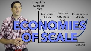
In long run costs, all inputs are considered variable, leading to the equivalence of total cost and total variable cost. The section introduces definitions and calculations for long run average cost (LRAC) and long run marginal cost (LRMC), highlighting their shapes and significance. It also discusses returns to scale and its impact on cost curves, stating that LRAC exhibits a U-shape guideline based on increasing and decreasing returns to scale.
Detailed
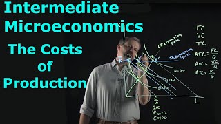
In the long run, all inputs to production can be varied, and hence, the total cost (TC) and total variable cost (TVC) converge, leading to a scenario where fixed costs are absent. Long run average cost (LRAC) is defined as the cost per unit of output, calculated as TC divided by output quantity (q). As output changes, the long run marginal cost (LRMC) reflects the change in total cost per change in output. The laws of returns to scale determine the behavior of LRAC; increasing returns to scale (IRS) imply decreasing average costs with larger outputs, while decreasing returns to scale (DRS) indicate increasing average costs. Typically, the LRAC curve appears 'U'-shaped, indicating decreasing average costs at low levels of production, transitioning to constant returns, and at higher levels experiencing increasing average costs.
Youtube Videos


Audio Book
Dive deep into the subject with an immersive audiobook experience.
Long Run Cost Definitions
Chapter 1 of 3
🔒 Unlock Audio Chapter
Sign up and enroll to access the full audio experience
Chapter Content
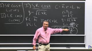
In the long run, all inputs are variable. There are no fixed costs. The total cost and the total variable cost therefore, coincide in the long run. Long run average cost (LRAC) is defined as cost per unit of output, i.e.
$$LRAC = \frac{TC}{q}$$
Long run marginal cost (LRMC) is the change in total cost per unit of change in output. When output changes in discrete units, then, if we increase production from $q_{1}$ to $q_{2}$ units of output, the marginal cost of producing the $q_{2}^{th}$ unit will be measured as
$$LRMC = TC_{at\,q_{2}} - TC_{at\,q_{1}}$$
Detailed Explanation
In the long run, a firm does not have any fixed costs, which means it can adjust all its inputs freely. As a result, the total cost (TC) and total variable cost (TVC) are the same in the long run. The Long Run Average Cost (LRAC) is calculated by dividing the total cost by the quantity of output produced. Similarly, the Long Run Marginal Cost (LRMC) measures how much the total cost changes when output increases by one unit, helping firms understand how much extra they will need to pay to produce more.
Examples & Analogies
Imagine a restaurant that can change its menu completely based on customer feedback. In the long run, they can adjust everything from the ingredients they buy (all inputs) to how many chefs they hire (labor). Instead of worrying about fixed costs (like rent), they can focus on how much it costs to serve each additional plate of food, making their operations more efficient.
Shapes of Long Run Cost Curves
Chapter 2 of 3
🔒 Unlock Audio Chapter
Sign up and enroll to access the full audio experience
Chapter Content
We have previously discussed the returns to scales. Now let us see their implications for the shape of LRAC.
IRS implies that if we increase all the inputs by a certain proportion, output increases by more than that proportion. In other words, to increase output by a certain proportion, inputs need to be increased by less than that proportion. With the input prices given, cost also increases by a lesser proportion. For example, suppose we want to double the output. To do that, inputs need to be increased, but less than double. The cost that the firm incurs to hire those inputs therefore also need to be increased by less than double. What is happening to the average cost here? It must be the case that as long as IRS operates, average cost falls as the firm increases output.
DRS implies that if we want to increase the output by a certain proportion, inputs need to be increased by more than that proportion. As a result, cost also increases by more than that proportion. So, as long as DRS operates, the average cost must be rising as the firm increases output.
CRS implies a proportional increase in inputs resulting in a proportional increase in output. So the average cost remains constant as long as CRS operates.
Detailed Explanation
Long Run Average Cost (LRAC) curves demonstrate how a firm's average cost evolves as it changes output levels. Under Increasing Returns to Scale (IRS), a firm can produce more output without having to proportionally increase its input costs, which causes average costs to decrease. Conversely, under Decreasing Returns to Scale (DRS), a firm needs to increase its input use more than proportionately to achieve higher output levels, leading to increased average costs. Constant Returns to Scale (CRS) means that when inputs are increased, output rises in the same proportion, keeping average costs stable.
Examples & Analogies
Consider a factory that manufactures bicycles. When they scale up production (IRS), they might find that by adding more assembly workers, they can produce a lot more bicycles without doubling their costs (like buying materials). However, once they hit a certain limit (DRS), adding more workers only adds a little to production and their costs skyrocket because they have to rent more space and buy more equipment. If everything goes perfectly balanced (CRS), then their costs remain stable as they add workers and equipment in equal measure.
Long Run Costs Visuals
Chapter 3 of 3
🔒 Unlock Audio Chapter
Sign up and enroll to access the full audio experience
Chapter Content
It is argued that in a typical firm IRS is observed at the initial level of production. This is then followed by the CRS and then by the DRS. Accordingly, the LRAC curve is a ‘U’-shaped curve. Its downward sloping part corresponds to IRS and upward rising part corresponds to DRS. At the minimum point of the LRAC curve, CRS is observed.
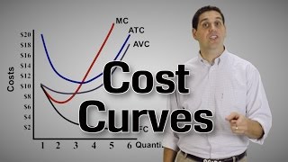
Let us check how the LRMC curve looks like. For the first unit of output, both LRMC and LRAC are the same. Then, as output increases, LRAC initially falls, and then, after a certain point, it rises. As long as average cost is falling, marginal cost must be less than the average cost. When the LRAC is rising, marginal cost must be greater than the average cost. LRMC curve is therefore a ‘U’-shaped curve. It cuts the LRAC curve from below at the minimum point of the LRAC.
Detailed Explanation
The Long Run Average Cost (LRAC) curve typically has a U-shape due to the stages of production scale a firm experiences. Initially, as production ramps up, firms enjoy decreasing costs (IRS). Once they reach an optimal level of production, costs stabilize (CRS), and if they continue to expand beyond capacity, costs begin to climb again (DRS). The Long Run Marginal Cost (LRMC) follows a similar U-shape pattern and intersects the LRAC at the lowest point, indicating the most efficient scale of production.
Examples & Analogies
Think of a chef opening a restaurant. At first, the chef can prepare more dishes efficiently (IRS), and their costs per dish decrease. After reaching a certain number of dishes, adding more cooks leads to more kitchen congestion (DRS), causing disorganization. The optimal number of dishes to serve signifies the LRAC's lowest point, where efficiency peaks—much like a well-timed dinner service!
Key Concepts
-
Long Run vs Short Run: In the long run, all inputs can be varied, unlike the short run where some are fixed.
-
LRAC Calculation: Long Run Average Cost (LRAC) is total cost divided by output quantity.
-
LRMC Definition: Long Run Marginal Cost (LRMC) is the change in total cost associated with producing one additional unit of output.
-
Returns to Scale: The degree to which output increases as inputs are increased.
Examples & Applications
If a firm can double its output by only increasing its inputs by 80%, it experiences increasing returns to scale.
A company with consistent production costs regardless of output level operates under constant returns to scale.
Memory Aids
Interactive tools to help you remember key concepts
Rhymes
In the long run, inputs are free, costs per output, clear to see.
Stories
Imagine a bakery. In short run, it uses fixed ovens. In long run, it builds more as demand grows, adjusting costs to stay profitable.
Memory Tools
LRAC = Total Costs / Quantity (Read as L-Q, like in school we solved for volume!).
Acronyms
TRC (Total, Runs, Costs) helps remember that total costs change over time as input factors vary.
Flash Cards
Glossary
- Long Run
A period during which all factors of production are variable.
- Long Run Average Cost (LRAC)
Cost per unit of output in the long run where total costs and total variable costs are identical.
- Long Run Marginal Cost (LRMC)
The change in total cost associated with the production of one additional unit in the long run.
- Returns to Scale
The rate at which production output increases in response to a proportional increase in all inputs.
Reference links
Supplementary resources to enhance your learning experience.