
Shapes of Total Product, Marginal Product and Average Product Curves
Enroll to start learning
You’ve not yet enrolled in this course. Please enroll for free to listen to audio lessons, classroom podcasts and take practice test.
Interactive Audio Lesson
Listen to a student-teacher conversation explaining the topic in a relatable way.
Total Product and its Curve
🔒 Unlock Audio Lesson
Sign up and enroll to listen to this audio lesson

Today, we're going to discuss Total Product, which refers to the total output produced by varying a single input while keeping all other inputs constant. Can anyone tell me what we mean by 'total product'?

Is it the overall amount of goods produced from the inputs used?
Exactly! For instance, if a factory uses varying amounts of labor, the total product measures how much output is generated from that labor. Does someone remember the relationship between total product and input variations?

Yes! More input generally leads to more output, but the rate may change?
Correct! That's crucial. This concept ties into our understanding of marginal product. Remember, total product increases after adding inputs, but not always at the same rate. Let's visualize this on a graph to grasp it better!
Average Product and its Relationship with Total Product
🔒 Unlock Audio Lesson
Sign up and enroll to listen to this audio lesson

Now that we understand total product, let’s discuss Average Product, or AP. Who can remind us how we define average product?

Average Product is the total product divided by the number of units of input used.
Spot on! AP essentially shows us the efficiency of our input usage. When we plot both the total product and average product on the same graph, how do you think they relate?

I think when total product increases, average product also tends to rise until it reaches a peak?
Exactly! This peak represents the highest efficiency of input. Let's remember—if total product is increasing but at a decreasing rate, average product can start declining as well.
Marginal Product and the Law of Diminishing Returns
🔒 Unlock Audio Lesson
Sign up and enroll to listen to this audio lesson
Let’s dive deeper into Marginal Product, or MP. How would you define it?
Marginal Product is the extra output gained from adding one more unit of input.
Exactly! The marginal product is key in understanding production efficiency. There’s something important called the law of diminishing returns. Who can explain what it means?
It means that after a certain point, adding more of one input leads to smaller increases in output.
Perfect! This concept is illustrated by the MP curve, which usually shows an inverse U-shape. Now, if we look at the graph of MP and AP together, what correlation do you see?
I think when MP is above AP, AP increases. But when MP falls below AP, then AP starts to decline.
Right! This interplay between MP and AP is very crucial for understanding production efficiency. Remember this relationship—it's often tested!
Graphical Representation of Product Curves
🔒 Unlock Audio Lesson
Sign up and enroll to listen to this audio lesson
Let's visualize the relationships we've discussed. If we graph Total Product, Average Product, and Marginal Product, what do we expect to see?
The TP curve should always go up, while the MP and AP curves will follow their own unique paths.
That's correct! The shape will help us visualize the efficiency of inputs over time, especially noticing where MP declines. What about the importance of these curves?
They help producers understand how efficiently they are using their resources and where they should allocate more or less!
Exactly! This understanding allows producers to maximize profits by optimizing input use. Let’s summarize what we've established about these curves today!
Introduction & Overview
Read summaries of the section's main ideas at different levels of detail.
Quick Overview
Standard
In this section, we explore the shapes of total product, marginal product, and average product curves in relation to input variations in the production process. The section discusses the implications of the law of variable proportions, showing how marginal product changes can affect the overall efficiency of production and how these curves are represented graphically.
Detailed
In production economics, the relationship between inputs and outputs can be represented through total product (TP), average product (AP), and marginal product (MP) curves. Total product reflects the output produced for varying levels of a single input while keeping other inputs constant. The average product indicates output per unit of variable input, calculated by dividing total product by the number of units of that input. Meanwhile, marginal product is the additional output generated by an additional unit of input.
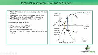
The section illustrates that as more labor is added (holding capital constant), total product increases at varying rates, leading to initially high marginal product that diminishes after a certain point due to the law of diminishing marginal product. Graphically, the TP curve slopes upward, while the MP curve takes an inverse 'U' shape, indicating that MP increases initially and then declines. In graphical representation, AP is influenced by MP; it rises when MP exceeds it and falls when MP is below it. This section emphasizes the importance of understanding these relationships to maximize production efficiency.
Youtube Videos


Audio Book
Dive deep into the subject with an immersive audiobook experience.
Understanding Total Product Curve
Chapter 1 of 4
🔒 Unlock Audio Chapter
Sign up and enroll to access the full audio experience
Chapter Content
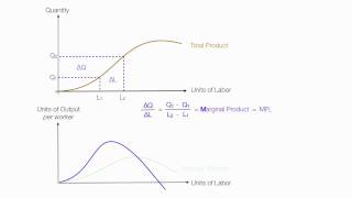
An increase in the amount of one of the inputs keeping all other inputs constant results in an increase in output. Table 3.2 shows how the total product changes as the amount of labour increases. The total product curve in the input-output plane is a positively sloped curve.
Detailed Explanation
The Total Product (TP) curve represents the relationship between the quantity of input used (in this case, labor) and the total output produced. When we use more labor while keeping other inputs the same, production typically increases. The curve slopes upwards because as more units of labor are employed, the output increases, indicating a positive relationship between input and output.
Examples & Analogies
Imagine a bakery where the amount of bread produced increases with additional bakers. If one baker bakes a certain number of loaves in an hour, adding another baker (while keeping the ovens and ingredients the same) will usually lead to more bread being baked. The total production would increase as more bakers join in.
Marginal Product Curve
Chapter 2 of 4
🔒 Unlock Audio Chapter
Sign up and enroll to access the full audio experience
Chapter Content
According to the law of variable proportions, the marginal product of an input initially rises and then after a certain level of employment, it starts falling. The MP curve therefore, looks like an inverse ‘U’-shaped curve.
Detailed Explanation
Marginal Product (MP) indicates the additional output generated by adding one more unit of input while keeping other inputs constant. Initially, as more labor is hired, each additional worker contributes significantly to output, thus increasing MP. However, after a certain point, the workplace may become crowded, and adding more workers leads to a decrease in the productivity of each worker due to limited space or resources, resulting in the MP curve eventually declining.
Examples & Analogies
Think of a classroom. At first, adding more students leads to richer discussions and learning. However, once the class gets too large, students may struggle to participate effectively, and additional students might hinder rather than help the learning process. This analogy illustrates the MP diminishing as the input (students) increases beyond an optimal level.
Average Product Curve
Chapter 3 of 4
🔒 Unlock Audio Chapter
Sign up and enroll to access the full audio experience
Chapter Content
Let us now see what the AP curve looks like. For the first unit of the variable input, one can easily check that the MP and the AP are the same. Now as we increase the amount of input, the MP rises. AP being the average of marginal products, also rises, but rises less than MP.
Detailed Explanation
The Average Product (AP) is calculated as the total output divided by the number of input units used. Initially, when additional inputs increase the output significantly, both the AP and MP rise. However, since AP is affected by the MP’s changes, it typically increases at a slower pace than MP due to averaging out the contributions from all previous one of inputs. An important point to note is that once MP falls below AP, AP begins to decline as well.
Examples & Analogies
Consider a sports team. Initially, adding star players increases the total team performance (output) significantly. However, as the team grows, some players may not contribute as much due to crowding on the field. While the total performance is high, the average contribution per player may start to decline, especially if their presence is not adding enough value.
Relationship Between AP and MP
Chapter 4 of 4
🔒 Unlock Audio Chapter
Sign up and enroll to access the full audio experience
Chapter Content
As long as the AP increases, it must be the case that MP is greater than AP. Otherwise, AP cannot rise. Similarly, when AP falls, MP has to be less than AP. It follows that the MP curve cuts the AP curve from above at its maximum.
Detailed Explanation
The relationship between Average Product (AP) and Marginal Product (MP) can be summarized by saying that MP influences AP. When MP is higher than AP, it raises the average, leading to an increasing AP. Conversely, when MP drops below AP, it pulls the average down, causing AP to decline. The point where MP intersects AP represents the peak average product.
Examples & Analogies
Imagine two chefs in a kitchen. If one chef can cook more dishes per hour than the average number of dishes cooked by both, the overall average (AP) increases. However, if one chef slows down due to fatigue, and their output falls below the average, the overall average output of dishes (AP) will decrease too.