
Applications of Integral Control
Enroll to start learning
You’ve not yet enrolled in this course. Please enroll for free to listen to audio lessons, classroom podcasts and take practice test.
Interactive Audio Lesson
Listen to a student-teacher conversation explaining the topic in a relatable way.
Introduction to Integral Control
🔒 Unlock Audio Lesson
Sign up and enroll to listen to this audio lesson

Today, we'll discuss Integral Control, which plays a vital role in eliminating steady-state errors. Can anyone tell me what they think steady-state error means?

Is it the difference that remains constant after several adjustments?
Exactly! Steady-state error is what remains after the system has stabilized. Integral control helps to eliminate this by integrating past errors over time. What might be a consequence of not addressing steady-state error?

The system would be less accurate in reaching the setpoint?
Correct! Integral control continuously adjusts the control signal to minimize this error.
Implementation Steps of Integral Control
🔒 Unlock Audio Lesson
Sign up and enroll to listen to this audio lesson

Let's discuss how we implement integral control. First, we measure the error. How do we calculate this error?

By subtracting the actual output from the desired setpoint?
Exactly! After measuring the error, we integrate it over time. Can someone explain how we might do this in software?

I think it can be done by summing up the errors at discrete time intervals.
Great! We then apply the integral gain, Ki, to the accumulated error to find our control input, u(t).
Applications of Integral Control
🔒 Unlock Audio Lesson
Sign up and enroll to listen to this audio lesson
Integral control is crucial in various applications. Can anyone provide examples where it may be used?
Temperature control in an oven?
Exactly! It ensures consistent temperature by addressing long-term deviations. What about in water systems?
It would help maintain the desired water level by adjusting inflow.
Exactly! However, we must be cautious of something known as integral windup. Can someone explain what that is?
Is it when the accumulated error gets too large and causes overshoot?
Right! Integral windup can lead to instability and requires careful management.
Challenges in Integral Control
🔒 Unlock Audio Lesson
Sign up and enroll to listen to this audio lesson
While integral control is beneficial, it has limitations. Who can name one?
Integral windup, when the error accumulates too much?
Exactly! This can lead to overshoot. What strategies might we use to prevent this?
We could limit the maximum value of the integral term?
Correct! Implementing anti-windup techniques helps manage this issue.
Recap and Key Takeaways
🔒 Unlock Audio Lesson
Sign up and enroll to listen to this audio lesson
Let's summarize today's lessons on integral control. What are the main advantages of using integral control?
It eliminates steady-state error!
And it can adjust for long-term deviation!
Excellent! Remember, while it can enhance system performance, we must also control for integral windup. Any last questions?
Can integral control be combined with other types?
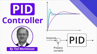
Yes! Often it's combined with proportional and derivative control to form a PID controller.
Introduction & Overview
Read summaries of the section's main ideas at different levels of detail.
Quick Overview
Standard
Integral control plays a critical role in applications where precision over time is essential, such as temperature and water level control. By accumulating past errors, integral control adjusts control inputs accordingly to nullify steady-state errors, but it can also lead to issues such as integral windup if not managed correctly.
Detailed
Integral control (I) is a feedback control strategy used to eliminate steady-state errors in systems by considering the accumulation of previous errors over time. Unlike proportional control, which addresses current error only, integral control integrates the error signal over time. This accumulation helps to adjust the control inputs (u(t)) dynamically, ensuring that persistent errors are progressively corrected. The integral gain (K_i) scales the accumulated error to calculate the control output.
Key Points Covered in this Section:
- Implementation Steps: Integral control necessitates measuring the error (difference between desired output and actual output), integrating this error over time, applying the integral gain, and adjusting the system based on the computed control input.
- Applications: Integral control is widely utilized for maintaining desired levels, such as in temperature regulation for ovens and water level management in tanks.
- Limitations: While integral control is effective, it can suffer from integral windup, where prolonged large errors lead to excessive control input, possibly causing instability or overshoot in system response.
Youtube Videos
Audio Book
Dive deep into the subject with an immersive audiobook experience.
Definition of Integral Control
Chapter 1 of 5
🔒 Unlock Audio Chapter
Sign up and enroll to access the full audio experience
Chapter Content
Integral Control (I) seeks to eliminate steady-state error by considering the accumulation of past errors. The integral action ensures that any persistent error over time results in a change in the control input, gradually driving the error to zero.
Detailed Explanation
Integral Control is a method used in control systems to correct errors over time by looking at the cumulative effect of past errors. Instead of just reacting to the current error, it sums the errors that have occurred. This accumulated error means that if the output of a system deviates from its target for a while, the control system will gradually adjust to bring it back to the correct level by modifying its control output progressively, thus eliminating any long-term steady-state errors.
Examples & Analogies
Imagine you are riding a bicycle. If you notice you are veering left, you correct your steering and lean slightly to the right. However, if you keep drifting left, that small adjustment becomes more significant over time, pushing you back on track. In this analogy, your constant corrections represent integral control, making larger adjustments if you continue to drift away from your intended path.
Mathematical Representation
Chapter 2 of 5
🔒 Unlock Audio Chapter
Sign up and enroll to access the full audio experience
Chapter Content
Mathematical Representation:
u(t)=Ki∫0te(τ)dτ
where:
● u(t) is the control input.
● Ki is the integral gain.
● e(t) is the error signal.
● The integral term accumulates the error over time, making corrections based on past errors.
Detailed Explanation
The mathematical representation of integral control shows how the control input (u(t)) is calculated as the integral of the error over time, multiplied by a constant known as the integral gain (Ki). This integral operation sums all the past error values from the start time up to the current time (t). By implementing this formula, a control system can adjust its output to correct any ongoing steady-state errors. 'Integrating the error' means continuously adding up the errors that have occurred over time, which eventually guides the control action to mitigate those errors.
Examples & Analogies
Think of a savings account where you add a small amount each month. At first, your balance grows slowly, but over time, those small amounts add up to create a substantial sum. In this case, the continuous addition of your savings is like the integral of past errors—it's a build-up that ultimately leads to a significant correction in your financial status.
Implementation Steps
Chapter 3 of 5
🔒 Unlock Audio Chapter
Sign up and enroll to access the full audio experience
Chapter Content
Implementation Steps:
1. Measure the error e(t) between the desired setpoint and actual output.
2. Integrate the error over time to accumulate the error (in software, this is typically implemented as a summation of discrete errors over each time step).
3. Apply the integral gain Ki to the accumulated error to compute the control input u(t).
4. Adjust the system (e.g., heating element, actuator) based on the control input.
Detailed Explanation
The implementation of integral control involves a specific sequence of actions:
1. First, measure the error between the desired output and what the system is currently producing.
2. Next, integrate this error over time (often in small steps) to accumulate the total past error.
3. Then, once this accumulated error is known, multiply it by the integral gain (Ki) to calculate the control input that needs to be applied.
4. Finally, implement this control input to modify the system's behavior, helping to drive the output towards the desired setpoint effectively.
Examples & Analogies
Consider a thermostat in your home. Initially, your room temperature is 68°F, but you want it at 72°F. The thermostat measures the error of 4°F (72°F - 68°F). Over a few minutes, if the heater continuously runs and hasn’t quite reached the target, it accumulates this error each minute, adjusting the heating output slightly each time until the temperature stabilizes at 72°F—hence the mechanism of integral control.
Applications of Integral Control
Chapter 4 of 5
🔒 Unlock Audio Chapter
Sign up and enroll to access the full audio experience
Chapter Content
Applications of Integral Control:
● Temperature Control: In systems like ovens or boilers, integral control ensures that long-term errors (e.g., small, persistent deviations in temperature) are corrected by increasing or decreasing heating power.
● Water Level Control: In tanks or reservoirs, integral control can be used to maintain the desired water level by adjusting inflow rates based on past deviations.
Detailed Explanation
Integral control is applied in various real-world situations where sustained offsets need correction. For instance, in heating systems such as ovens, if there is a consistent underheating (e.g., always 1°F less than the set temperature), integral control adjusts the heating power over time to recover from this error. Similarly, in water reservoir systems, if the water levels drop below a set target, integral control can increase the inflow gradually based on the cumulative decline in levels, keeping the system stabilized at the desired level.
Examples & Analogies
Imagine a slow leak in a swimming pool. If the water has been consistently falling due to this leak, the pool maintenance system needs to regularly adjust the water supply, based on how much water has been lost over days. This gradual adjustment resembles integral control, where persistent past errors (water levels dropping) are corrected ably without causing drastic changes that might overflow the pool.
Limitations of Integral Control
Chapter 5 of 5
🔒 Unlock Audio Chapter
Sign up and enroll to access the full audio experience
Chapter Content
Limitations:
● Integral windup: If the error is large for an extended period, the integral term can grow excessively (integral windup), leading to instability or overshoot.
Detailed Explanation
One significant limitation of integral control is a phenomenon called 'integral windup.' This occurs when there is a large and persistent error in the system. As the errors accumulate, the control output may grow excessively large, leading to overshooting the desired setpoint and possibly causing instability in the system. Essentially, if the control input becomes too high due to the accumulated value of the errors, the system might overcorrect, leading to oscillations or even failure to stabilize.
Examples & Analogies
Think of a car's accelerator. If you have your foot on the pedal and you're driving up a steep hill, the car may not get enough power due to the angle. You might continuously press the pedal harder (accumulating error), but if you don't ease off once you reach level ground, the car might speed uncontrollably, leading to a scenario where you're overcorrecting and losing control. This is akin to the challenges faced with integral windup in control systems.
Key Concepts
-
Integral Control: A feedback strategy that uses accumulated past error to eliminate steady-state error.
-
Accumulated Error: The total error integrated over time, impacting control adjustments.
-
Integral Gain: A coefficient that scales the accumulated error for effective control input calculation.
-
Applications: Integral control is used in systems like temperature regulation and liquid level control.
-
Integral Windup: A condition where excessive error accumulation leads to instability.
Examples & Applications
In a heating system, integral control adjusts the heating element power based on past temperature errors to ensure the desired temperature is consistently achieved.
In a reservoir system, integral control manages the inflow based on historical water level errors, maintaining the desired level without overshooting.
Memory Aids
Interactive tools to help you remember key concepts
Rhymes
To keep the system steady, integrate and be ready; past errors yield control, making outputs whole!
Stories
Once, a baker struggled with his oven's temperature. He learned to collect the temperature errors over time, ensuring cake perfection without burning, thanks to integral control!
Memory Tools
I for Integral, E for Elimination of Error, A for Accumulation of past mistakes.
Acronyms
I.C.E. - Integral controls Eliminates error.
Flash Cards
Glossary
- Integral Control
A control strategy that accumulates past error values to eliminate steady-state errors in control systems.
- SteadyState Error
The persistent difference between the desired setpoint and the actual output of a control system after it has settled.
- Integral Windup
A condition in which the accumulation of error in integral control leads to excessive control action, potentially causing system instability.
- Integral Gain (K_i)
The coefficient applied to the accumulated error in integral control to calculate the control input.
- Control Input (u(t))
The resulting input signal to the system based on the control strategy employed.
Reference links
Supplementary resources to enhance your learning experience.