
Derivative Control (D)
Enroll to start learning
You’ve not yet enrolled in this course. Please enroll for free to listen to audio lessons, classroom podcasts and take practice test.
Interactive Audio Lesson
Listen to a student-teacher conversation explaining the topic in a relatable way.
Introduction to Derivative Control
🔒 Unlock Audio Lesson
Sign up and enroll to listen to this audio lesson

Today we're diving into Derivative Control, or simply 'D' control. Can anyone tell me what they think the role of Derivative Control is in a system?

Is it about predicting future errors based on the current error?
Exactly, Student_1! Derivative Control predicts future errors by looking at how quickly the current error is changing. This way, it can act before the error gets too large.

So, it helps minimize overshoot?
Yes, precisely! By taking into account the rate of change, it helps dampen oscillations in systems. We must balance the control input carefully to avoid instability due to noise, though. Let's remember: **D = Do Future Planning**. Can anyone recall what that means?

It means we should consider the future behavior of errors!
Correct! Great engagement!
Mathematical Representation
🔒 Unlock Audio Lesson
Sign up and enroll to listen to this audio lesson

Now, let's look at the mathematical representation of Derivative Control. Can someone summarize it for us?
It's u(t) = Kd * d/dt e(t), right?
That's correct! Here, **u(t)** is the control input and **K_d** is the derivative gain. Why do you think the derivative term is useful?
It helps predict how quickly the error is changing!

And it helps to adjust the control input before big errors happen!
Absolutely! It's crucial in maintaining stability in fast-changing processes. Let's remember the formula: **u(t) = Kd * d/dt e(t)**. Can someone explain what **K_d** does?
It's how sensitive the system's response is to changes in error!
Exactly! Well done, everyone!
Applications of Derivative Control
🔒 Unlock Audio Lesson
Sign up and enroll to listen to this audio lesson
Let's move on to applications! Where can we see Derivative Control used in real-world scenarios?
I think it's in motor control systems to smooth out transitions?
Correct! Motor controls benefit significantly from D control for managing speed and position efficiently. Any other examples?
What about in vibration control for cars?
Exactly, Student_1. Vibration control systems also use Derivative Control to dampen oscillations caused by road irregularities. Let’s keep that in mind. A good way to remember is: **Damping Delay in Dynamics - DDD**. Can anyone explain that?
It's to remember that D control helps delay the effects of sudden changes!
Right! Excellent job!
Limitations of Derivative Control
🔒 Unlock Audio Lesson
Sign up and enroll to listen to this audio lesson
Now let's touch upon some limitations. What do you think could be a downside of Derivative Control?
Isn't it sensitive to noise in the error signal?
That's spot on! The noise in the error can cause the control input to fluctuate rather than stabilize. This can lead to instability in the system. We need a way to recall this aspect. How can we summarize it?
Maybe something like **Dangerously Sensitive to Disturbances - DSD**?
Great mnemonic, Student_2! Additionally, implementing filtering techniques can help reduce noise effects. Any other thoughts on its limitations?
Can large errors lead to unexpected responses too?
Absolutely, this is another crucial point! Avoid large error scenarios whenever possible. Well done today!
Introduction & Overview
Read summaries of the section's main ideas at different levels of detail.
Quick Overview
Standard
In Derivative Control, the focus is on evaluating how quickly the error is changing. By utilizing this rate of change, control systems can effectively dampen oscillations and improve response stability, particularly important in dynamic environments like motor controls and mechanical systems. However, care must be taken due to its sensitivity to signal noise.
Detailed
Detailed Summary
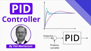
In this section, we explore Derivative Control (D), a key feedback control method crucial in managing system behaviors, particularly where preventing overshoot and oscillation is essential. Derivative Control responds not just to the current error between the desired output and actual output but also to the rate at which this error is changing. Mathematically, the control input is represented as:
\[ u(t) = K_d \cdot \frac{d}{dt} e(t) \]
Here, u(t) is the control input, K_d is the derivative gain, and e(t) is the error signal. The control law's significance lies in its application to various engineering fields, such as motor control systems where it helps ensure smooth and controlled transitions, and vibration control systems where it dampens undesired oscillations. However, one major limitation is the algorithm's sensitivity to noise, which can result in erratic control actions in the presence of high-frequency fluctuations. This section emphasizes the fundamental aspects of Derivative Control, its implementation steps, real-world applications, and associated limitations.
Youtube Videos
Audio Book
Dive deep into the subject with an immersive audiobook experience.
Overview of Derivative Control
Chapter 1 of 5
🔒 Unlock Audio Chapter
Sign up and enroll to access the full audio experience
Chapter Content
Derivative Control (D) predicts the future error by considering the rate of change of the error. By responding to how fast the error is changing, derivative control helps to minimize overshoot and dampen oscillations in the system.
Detailed Explanation
Derivative control is a strategy that predicts what will happen to the error in the future, based on how quickly the error itself is changing. This means that instead of just looking at how far off we are from our desired outcome (the error), we also consider how quickly that error is increasing or decreasing. In simple terms, if you’re driving a car and you notice you’re speeding up towards a red light, derivative control helps you to stop speeding too much before you get to the light, reducing sudden stops.
Examples & Analogies
Imagine you are baking bread. You can’t only rely on how much the dough has risen (the current error), but you also need to monitor how fast it’s rising. If it’s rising quickly, you might need to adjust the temperature right away to avoid overflowing. That’s how derivative control works; it keeps you from making drastic changes that could disrupt the baking process.
Mathematical Representation
Chapter 2 of 5
🔒 Unlock Audio Chapter
Sign up and enroll to access the full audio experience
Chapter Content
Mathematical Representation:
u(t)=Kd⋅ddte(t)u(t) = K_d \cdot \frac{d}{dt} e(t)
where:
● u(t)u(t) is the control input.
● KdK_d is the derivative gain.
● e(t)e(t) is the error signal.
● The derivative term responds to the rate of change of the error.
Detailed Explanation
In the mathematical representation of derivative control, 'u(t)' represents the control input we want to apply to the system at time 't'. The term 'K_d' is the derivative gain, which determines how much we react to the change rate of the error. The expression 'ddte(t)' calculates the rate of change of the error, meaning we are looking at how fast 'e(t)', the difference between the desired and actual system output, is changing. Thus, this formula allows the controller to respond not just based on how far off we are, but how quickly that distance is changing.
Examples & Analogies
Think of this like a speedometer in a car. The amount of pressure you need to apply to the brakes (control input, 'u(t)') isn’t just based on how fast you’re going (the current speed, 'e(t)') but also on how quickly your speed is increasing or decreasing (the rate of change). If you’re going downhill rapidly, you need to press harder on the brakes than if you’re just cruising on a flat road.
Implementation Steps
Chapter 3 of 5
🔒 Unlock Audio Chapter
Sign up and enroll to access the full audio experience
Chapter Content
Implementation Steps:
1. Measure the error e(t)e(t) and its rate of change ddte(t)\frac{d}{dt} e(t).
2. Calculate the derivative of the error, often approximated in discrete systems as the difference between current and previous errors.
3. Multiply the derivative by the gain KdK_d to compute the control input.
4. Apply the control input to the system to counteract rapid changes in error.
Detailed Explanation
To implement derivative control involves several steps. First, we need to measure the current error and how quickly that error is changing. This gives us the necessary data. Second, we approximate how much the error has changed by comparing the error now with the error from a previous moment. Third, this change is multiplied by the derivative gain ('K_d') to find out how much we need to adjust our control input. Finally, we apply this control input to the system to help stabilize it quickly, reducing any rapid changes we observe in the error.
Examples & Analogies
Picture a roller coaster. As you ascend, you feel the anticipation (the error), and once on top, the speed changes (the rate of change). If you suddenly start dropping, the operator must react quickly to smooth the ride for everyone. They measure how fast the coaster is descending, decide on the right brakes to apply, and then enact it to ensure a smoother experience. Each step is crucial for a safe ride.
Applications of Derivative Control
Chapter 4 of 5
🔒 Unlock Audio Chapter
Sign up and enroll to access the full audio experience
Chapter Content
Applications of Derivative Control:
● Motor Control: Derivative control can be used in DC motors or servos to dampen oscillations and smooth out transitions when adjusting position or speed.
● Vibration Control: In mechanical systems like suspension systems, derivative control helps in damping oscillations caused by external disturbances.
Detailed Explanation
Derivative control has various practical applications. In motor control systems, it helps reduce the wobbling and fluctuations that may occur when a motor is trying to reach a new speed or position, ensuring smoother operation. In mechanical systems, like vehicle suspensions, it plays a vital role in absorbing shocks from bumps on the road, which is crucial for stability and comfort. Essentially, where control needs to manage quick changes and oscillations, derivative control is often implemented.
Examples & Analogies
Think about driving a car over a bumpy road. The suspension system (that uses derivative control principles) helps to absorb the bumps and maintain a smooth ride. If it wasn't there, every bump would jolt you back and forth dramatically. Instead, the suspension gently reacts to those bumps, smoothing the ride out much like how derivatives manage changes in errors smoothly.
Limitations of Derivative Control
Chapter 5 of 5
🔒 Unlock Audio Chapter
Sign up and enroll to access the full audio experience
Chapter Content
Limitations:
● Noise Sensitivity: Derivative control can be very sensitive to noise in the error signal, as small fluctuations in error will result in large control inputs.
Detailed Explanation
While derivative control is very useful, it does have limitations. One of the primary issues is its sensitivity to noise in the measurement of the error signal. If there are small fluctuations caused by interference or inaccuracies in measuring the error, derivative control will react strongly to these noise signals, potentially leading to overly aggressive control actions. This means that instead of stabilizing the system, it might cause erratic behavior.
Examples & Analogies
Imagine trying to balance a delicate stack of books while someone keeps bumping the table (the noise). As soon as you detect a shift (the error signal), you might instinctively overreact and try to adjust too aggressively in the other direction. Instead of stabilizing, your movements could end up destabilizing the stack even more. That’s the kind of issue derivative control faces with noisy signals.
Key Concepts
-
Rate of Change: Derivative Control helps anticipate future errors by analyzing how the current error is changing.
-
Response Stability: By predicting changes, Derivative Control minimizes overshoot and enhances system stability.
-
Noise Sensitivity: Derivative Control can be highly sensitive to noise, making systems erratic.
-
Real-World Applications: Used in motor control and vibration damping, showcasing its practicality.
Examples & Applications
In motor control, Derivative Control is used to smooth out the speed transition of DC motors.
In the automotive sector, it helps control vibrations in suspension systems to ensure a smoother ride.
Memory Aids
Interactive tools to help you remember key concepts
Rhymes
In systems that twist and turn, Derivative Control is what we learn; it dampens the change, smooths the ride, keeping systems safe inside.
Stories
Imagine a tightrope walker adjusting quickly to maintain balance, just as Derivative Control adjusts to changing errors to keep a system stable.
Memory Tools
Remember PRIME: Predict, Respond, Improve, Minimize, Enhance - key steps in Derivative Control.
Acronyms
DAMP
Derivative approaches manage predictions to dampen overshoot.
Flash Cards
Glossary
- u(t)
The control input in Derivative Control, determined by the derivative of the error signal.
- Kd
The derivative gain, which determines the system's response sensitivity to the error change rate.
- e(t)
The error signal, the difference between the desired and actual outputs.
- Overshoot
The phenomenon where a control system exceeds its target value before settling.
- Oscillation
Fluctuations of the output variable around the target value after overshoot.
- Noise
Unwanted disturbances that can affect the signals within control systems.
Reference links
Supplementary resources to enhance your learning experience.