
Mathematical Representation - 10.4.1
Enroll to start learning
You’ve not yet enrolled in this course. Please enroll for free to listen to audio lessons, classroom podcasts and take practice test.
Interactive Audio Lesson
Listen to a student-teacher conversation explaining the topic in a relatable way.
Proportional Control
🔒 Unlock Audio Lesson
Sign up and enroll to listen to this audio lesson

Today, we begin with Proportional Control. Can anyone tell me what Proportional Control is?

Isn't that when the control input is directly proportional to the error?
Exactly! The control input is calculated using the formula: \(u(t) = K_p imes e(t)\), where \(K_p\) is the proportional gain. The error \(e(t)\) is the difference between the desired setpoint and current output. This means if the error increases, the control input will increase as well.

Can it fully eliminate the error?
Good question! While it adjusts the control input according to the error, Proportional Control cannot eliminate steady-state error. It stabilizes at some error level based on \(K_p\).

What are some practical applications of this control?
Great observation! Common applications include motor speed control and thermostats. In these cases, adjustments are made to ensure outputs remain close to the desired setpoint.

What happens if \(K_p\) is very high?
Higher \(K_p\) can lead to an aggressive control response, potentially causing system instability. In summary, Proportional Control is crucial for adjusting outputs based on immediate errors.
Integral Control
🔒 Unlock Audio Lesson
Sign up and enroll to listen to this audio lesson

Let's move on to Integral Control. Why do you think we need an integral component in our control systems?
To deal with steady-state error?
Absolutely! Integral Control accumulates past errors to eliminate steady-state error. The formula is \(u(t) = K_i \int_0^t e(\tau) d\tau\). Can anyone explain this integral term?
It builds up the error over time?
Correct! It means the longer there's an error, the more impact it has on the control input. However, we must be careful of 'integral windup.' What do you think could happen?
It could lead to overshooting the target?
Exactly! Maintaining a balance is key, and applications like water level control in tanks benefit significantly from integral action.
Derivative Control
🔒 Unlock Audio Lesson
Sign up and enroll to listen to this audio lesson
Now let's talk about Derivative Control. What role do you think it plays in controlling systems?
I think it helps predict future errors?
Precisely! The formula is \(u(t) = K_d \frac{d}{dt} e(t)\). By looking at the rate of change of error, it helps to minimize overshoot. Why is that important?
It keeps the system stable?
Exactly! However, this type of control can be sensitive to noise. What might be a solution to this problem?
We can filter the error signal?
Correct! Derivative Control is crucial for applications like motor control and reducing oscillations in mechanical systems.
PID Control
🔒 Unlock Audio Lesson
Sign up and enroll to listen to this audio lesson
Finally, let’s discuss PID Control. Why might we combine all three controls into one?
To take advantage of all their strengths?
Exactly! The equation reads: \(u(t) = K_p imes e(t) + K_i \int_0^t e(\tau) d\tau + K_d \frac{d}{dt} e(t)\). How does this solution improve system performance?
It provides both instantaneous correction and long-term stability!
Correct! This combination is widely applied in HVAC systems, motor controls, and many more applications. Tuning the PID parameters is crucial – can anyone name a tuning method?
The Ziegler-Nichols Method!
Great recall! In conclusion, PID Control optimally handles varied conditions providing a robust solution in control systems.
Introduction & Overview
Read summaries of the section's main ideas at different levels of detail.
Quick Overview
Standard
The section provides an overview of the mathematical formulas that define key control laws in engineering. It emphasizes the Proportional (P), Integral (I), Derivative (D), and PID control mechanisms, detailing their equations, implementation steps, applications, and limitations, setting the stage for practical applications in real-world scenarios.
Detailed
Mathematical Representation
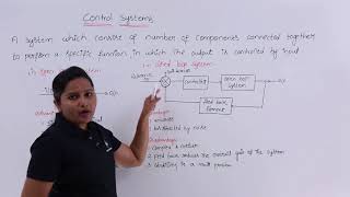
This section delves into the mathematical representation crucial for understanding control laws used in engineering systems. Control laws such as Proportional (P), Integral (I), Derivative (D), and PID (Proportional-Integral-Derivative) form the backbone of controlling system behaviors in various applications, including robotics, automotive systems, and process control.
Key Points:
- Proportional Control (P): The control input is calculated based on the current error derived from the setpoint and actual output. The equation is given by:
$$u(t) = K_p imes e(t)$$
where \(u(t)\) is the control input, \(K_p\) is the proportional gain, and \(e(t) = r(t) - y(t)\) is the error signal.
- Integral Control (I): This approach considers the accumulated error over time to work towards eliminating steady-state error with the equation:
$$u(t) = K_i \int_0^t e(\tau) d\tau$$
Here, \(K_i\) is the integral gain.
- Derivative Control (D): This predicts future error based on the rate of change of error:
$$u(t) = K_d \frac{d}{dt} e(t)$$
where \(K_d\) is the derivative gain.
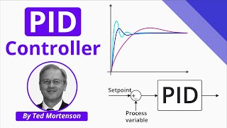
- PID Control: By combining P, I, and D control, this algorithm effectively minimizes error, eliminates steady-state error, and prevents overshoot. The equation is:
$$u(t) = K_p \cdot e(t) + K_i \int_0^t e(\tau) d\tau + K_d \frac{d}{dt} e(t)$$
Significance:
Understanding these mathematical representations provides the foundational knowledge necessary for the practical implementation of control laws in real-world engineering applications.
Youtube Videos
Audio Book
Dive deep into the subject with an immersive audiobook experience.
Control Input Definition
Chapter 1 of 3
🔒 Unlock Audio Chapter
Sign up and enroll to access the full audio experience
Chapter Content
u(t)=Kd⋅ddte(t)u(t) = K_d imes rac{d}{dt} e(t)
Detailed Explanation
In the equation provided, 'u(t)' represents the control input to the system. This input is influenced by the derivative of the error signal. The error signal 'e(t)' is the difference between the desired output and the actual output of the system. The term 'Kd' (K_d) represents the derivative gain, which determines how strongly the control input reacts to the change in error.
Examples & Analogies
Imagine a car that's trying to maintain a constant speed. The driver's input (the accelerator pedal) is analogous to the control input 'u(t)', while the difference between the current speed and the desired speed represents the error signal 'e(t)'. The quicker the speed is changing, the more the driver needs to adjust the accelerator based on how fast the car is speeding up or slowing down, which connects to the concept of the derivative gain.
Error Signal Explanation
Chapter 2 of 3
🔒 Unlock Audio Chapter
Sign up and enroll to access the full audio experience
Chapter Content
where: ● u(t)u(t) is the control input. ● KdK_d is the derivative gain. ● e(t)e(t) is the error signal.
Detailed Explanation
The error signal 'e(t)' is crucial because it shows how far off the system's output is from the desired target. For example, if a thermostat is set to 70°F but the actual temperature is 68°F, the error signal e(t) would be (70 - 68) = 2°F. The derivative gain 'Kd' is a coefficient that adjusts the response to this error's rate of change. A higher value of Kd means that the controller will act more aggressively to changes in the error signal.
Examples & Analogies
Think of a temperature control system: if it's cold outside and the heating takes too long to respond, the error signal reveals why it needs to do more. If we adjust the 'Kd' to be higher, it will quickly react to the increasing gap, ensuring the house warms up faster before it even reaches that chilly point.
Rate of Change of Error
Chapter 3 of 3
🔒 Unlock Audio Chapter
Sign up and enroll to access the full audio experience
Chapter Content
● The derivative term responds to the rate of change of the error.
Detailed Explanation
The derivative term plays a significant role in determining how quickly the control system should respond to changes. If the error is decreasing rapidly, the derivative control can minimize overshoot by calculating how fast that error is changing. Essentially, it anticipates the future behavior of the system based on how the error is changing, creating a smoother adjustment rather than reacting too harshly or slowly.
Examples & Analogies
Consider a dancer on stage who needs to adjust their movements based on the audience's reaction. If they sense that the applause is diminishing, they might pick up their pace or change their routine to re-engage the audience. Here, the 'rate of change of applause' can be likened to the derivative of the error: it's about quickly adjusting movements based on the audience's reaction to maintain an engaging performance.
Key Concepts
-
Proportional Control: Control input based on current error.
-
Integral Control: Addresses steady-state error through accumulated error.
-
Derivative Control: Predicts future error using the rate of change.
-
PID Control: Combined method providing robust system management.
Examples & Applications
A thermostat uses Proportional Control to adjust heating power based on temperature errors.
An automotive cruise control system employs PID Control to maintain vehicle speed.
Memory Aids
Interactive tools to help you remember key concepts
Rhymes
To adjust your control in a swift and precise way, use Kp, Ki, Kd each day.
Stories
Imagine a driver tuning their car. The Proportional Control is their immediate response to speed, the Integral Control is their adjustment over a long journey, and the Derivative Control is their careful watch on curves ahead.
Memory Tools
Remember PID as 'Pretty Intelligent Driver' controlling the car speed - reacting now, learning from the past, and anticipating turns.
Acronyms
Use PIDA - Predictive, Immediate, Derivative, Action - to recall the concepts.
Flash Cards
Glossary
- Control Input
The output provided by a control algorithm to influence system behavior.
- SteadyState Error
The persistent error that occurs in a system when it reaches a steady state.
- Proportional Gain (Kp)
A tuning parameter that scales the control input based on current error.
- Integral Gain (Ki)
A tuning parameter that affects how the accumulated error impacts the control input.
- Derivative Gain (Kd)
A tuning parameter that influences the control input based on the rate of change of the error.
- Integral Windup
A condition where the integral term accumulates excessively, leading to potential instability.
- PID Control
A control strategy that combines Proportional, Integral, and Derivative actions to optimally manage system behavior.
Reference links
Supplementary resources to enhance your learning experience.