
Implementation Steps - 10.5.2
Enroll to start learning
You’ve not yet enrolled in this course. Please enroll for free to listen to audio lessons, classroom podcasts and take practice test.
Interactive Audio Lesson
Listen to a student-teacher conversation explaining the topic in a relatable way.
Understanding Proportional Control
🔒 Unlock Audio Lesson
Sign up and enroll to listen to this audio lesson

Today, we'll dive into implementing Proportional Control. Can someone tell me what Proportional Control involves?

It adjusts the control input based on the error between the desired setpoint and the actual output!
That's correct! Let's go over the steps. First, we determine the desired setpoint, right? What comes next?

We measure the output using sensors to see the current performance of the system.
Exactly! And then we calculate the error. Who can remind us how we compute the error?

It's the difference between the setpoint and the output—e(t) = r(t) - y(t)!
Great job! After calculating the error, what do we do next?

We multiply the error by the proportional gain to get the control input!
Spot on! This helps us apply the control input to the system. Remember, for Proportional Control, the acronym PECA might help: Compute the error, Obtain the control input, and Apply it. Let's summarize what we've learned.
1) Determine setpoint, 2) Measure output, 3) Calculate error, 4) Calculate control input, 5) Apply control. Excellent work!
Implementing Integral Control
🔒 Unlock Audio Lesson
Sign up and enroll to listen to this audio lesson

Now let's move to Integral Control. What distinguishes it from Proportional Control?
It considers the accumulation of past errors to eliminate steady-state error!
Excellent! So can anyone list the steps we need to follow for Integral Control?
First, we measure the error, then we integrate it over time.
Correct! The cumulative errors allow us to compute the control input. What do we do after that?
We apply the integral gain to the accumulated error to determine the control input!
Yes, and finally, we apply this control input back into the system. Now let’s not forget a potential limitation: what is 'Integral Windup'?
It's when the integral term grows too large during significant error periods, causing instability!
Exactly! Let's sum up Integral Control's steps: Measure error, Integrate error, Calculate control input, Apply control. Remember the acronym MICA for these steps!
Understanding Derivative Control
🔒 Unlock Audio Lesson
Sign up and enroll to listen to this audio lesson
Next, we will focus on Derivative Control. How does this type of control aid system stability?
It predicts future errors by looking at the rate of change of the current error. This smooths out responses!
Good point! Can anyone walk me through the steps we take in Derivative Control?
First, we measure the error and its rate of change.
Correct! What comes after this initial measurement?
We calculate the derivative of the error!
Right! This determines how quickly the error is changing. What do we do next?
We multiply the derivative by the derivative gain to compute the control input!
Exactly! Finally, we apply this control input to the system. Derivative Control is sensitive to noise though. Can anyone explain why?
Because small fluctuations in the error can lead to large swings in control inputs!
Correct! So, let's sum up the steps: Measure error, Calculate derivative, Compute control input, Apply control. You can remember it by the acronym MDCA!
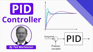
Combining Controls with PID Control
🔒 Unlock Audio Lesson
Sign up and enroll to listen to this audio lesson
Lastly, let's tie everything together by looking at PID Control. What makes PID control special?
It combines Proportional, Integral, and Derivative controls into one system!
Absolutely! Let's outline the steps for PID Control. Who's ready?
We start by measuring the error.
Then, we compute each of the P, I, and D terms!
Exactly! We combine those to find the total control input. Can anyone share the formulation?
u(t) = Kp * e(t) + Ki * ∫0t e(τ)dτ + Kd * ddte(t)!
Perfect! And finally, we apply the control input—this gives us a robust control mechanism. Remember the key applications of PID control!
Like temperature control in HVAC systems or speed control in motors!
Exactly! Let's conclude the session by summarizing the PID steps: Measure error, Compute P, I, D terms, Combine, and Apply control. An acronym to remember these is MICCA!
Introduction & Overview
Read summaries of the section's main ideas at different levels of detail.
Quick Overview
Standard
Implementation steps for control laws are vital for ensuring systems respond accurately to inputs. Each type of control law—Proportional, Integral, Derivative, and PID—has unique steps that detail how to determine errors, compute control inputs, and apply these in practical systems.
Detailed
Implementation Steps
Overview
In the implementation of control laws, engineers follow specific steps tailored to each control type. Here we focus on Proportional (P), Integral (I), Derivative (D), and PID (Proportional-Integral-Derivative) control laws. Each of these implementation steps is critical for transforming theoretical concepts into functioning control systems in practical applications such as robotics, automotive systems, and process control.
Proportional Control Steps
- Determine the desired setpoint (r(t)): Identify the target value the system should achieve.
- Measure the output (y(t)): Use sensors to capture the system's current output.
- Calculate the error (e(t)): Compute the error as the difference between the setpoint and the output (e(t) = r(t) - y(t)).
- Determine control input (u(t)): Calculate the control action by multiplying the error by the proportional gain (u(t) = Kp * e(t)).
- Apply the control: Implement the control input in the system.
Key Applications
- Motor Speed Control: Adjusts voltage based on speed error to maintain optimal motor performance.
- Thermostat Control: Regulates heating elements to maintain desired temperatures.
Integral Control Steps
- Measure the error (e(t)): Capture the difference between setpoint and output.
- Integrate the error: Accumulate past errors typically using numerical summation.
- Calculate control input (u(t)): Apply integral gain to this accumulated error (u(t) = Ki * ∫0t e(τ)dτ).
- Adjust the system: Implement the control input for system correction.
Key Applications
- Long-term Temperature Regulation: Ensures temperature corrections for systems with persistent discrepancies.
- Water Level Control: Adjusts inflow in reservoirs based on previous errors.
Derivative Control Steps
- Measure current error (e(t)): Determine present error values.
- Calculate rate of change: Compute the derivative of the error signal.
- Calculate control input (u(t)): Multiply derivative by the derivative gain to finalize control input.
- Apply control: Implement adjustments to counter rapid changes in error.
Key Applications
- Damping Oscillations in Motors: Smooth transitioning for precise operation in motor control systems.
- Suspension Systems: Reduces oscillation effects in mechanical designs.
PID Control Steps
- Measure error (e(t)): Determine the current system error.
- Compute P, I, D terms: Calculate the proportional, integral, and derivative contributions.
- Combine terms: Calculate total control input (u(t) = Kp * e(t) + Ki * ∫0t e(τ)dτ + Kd * ddte(t)).
- Apply control: Implement the determined control input in the system.
Key Applications
- HVAC Systems: Maintain precise control of temperatures.
- Robot Positioning: Enhance accuracy in robotic systems.
Youtube Videos
Audio Book
Dive deep into the subject with an immersive audiobook experience.
Measuring the Error
Chapter 1 of 4
🔒 Unlock Audio Chapter
Sign up and enroll to access the full audio experience
Chapter Content
- Measure the error e(t)e(t) in the system.
Detailed Explanation
The first step in implementing a PID controller is to measure the error in the system. The error is defined as the difference between the desired setpoint (the target value you want to achieve) and the actual output of the system. This error is critical because it informs the controller how far off the current output is from where it should be. Accurate measurement of this error is essential for effective control.
Examples & Analogies
Imagine you’re trying to fill a bathtub with water to a specific height (the setpoint). The actual water level is measured using a water level indicator (like a marked stick or a float). The difference between where you want the water level to be and where it currently is represents your error.
Computing Control Terms
Chapter 2 of 4
🔒 Unlock Audio Chapter
Sign up and enroll to access the full audio experience
Chapter Content
- Compute the proportional, integral, and derivative terms.
Detailed Explanation
In this step, you use the measured error to calculate the three components of PID control: the proportional term, the integral term, and the derivative term. Each term serves a different purpose: the proportional term responds to the current error, the integral term considers the accumulated past errors, and the derivative term anticipates future errors based on the rate of change of error. The combination of these three terms helps create a balanced control input that effectively corrects the system's output.
Examples & Analogies
Think of a driver trying to keep a car at a specific speed. The proportional term is like the driver pressing the accelerator based on the current speed difference. The integral term is like the driver remembering how long they've been below the speed limit, gradually pressing harder to compensate. The derivative term is akin to the driver anticipating the need to ease off the gas as they gain speed quickly, so they don’t overshoot the limit.
Calculating the Control Input
Chapter 3 of 4
🔒 Unlock Audio Chapter
Sign up and enroll to access the full audio experience
Chapter Content
- Combine the terms to calculate the control input u(t)u(t).
Detailed Explanation
After calculating the proportional, integral, and derivative terms, the next step is to combine these terms to compute the control input, denoted as u(t). This input represents the corrective action that will be applied to the system. The formula used typically looks like this: u(t) = Kp * e(t) + Ki * ∫ e(t) dt + Kd * (de(t)/dt). This comprehensive input is designed to minimize the error effectively based on present, past, and predicted future behavior of the system.
Examples & Analogies
If we return to our car example, the control input u(t) could be seen as the driver adjusting the throttle. The proportional response adjusts how much gas is applied based on current speed, the integral keeps track of the overall speed history (leading to adjustments if you've been slow for a while), and the derivative predicts how quickly the car is gaining speed, preventing it from going too fast.
Applying Control Input to the System
Chapter 4 of 4
🔒 Unlock Audio Chapter
Sign up and enroll to access the full audio experience
Chapter Content
- Apply the control input to the system.
Detailed Explanation
The final step in the implementation process is to apply the calculated control input to the system. This action may involve physical outputs, such as adjusting the power to a heater, changing the speed of a motor, or altering the position of a valve. The goal here is to actively implement the correction that will bring the system closer to the desired setpoint based on the indicated control input.
Examples & Analogies
Continuing with the car analogy, applying the control input is like the driver pressing down on the accelerator to increase speed or easing off to slow down. The immediate feedback from the car's speed helps the driver adjust the throttle as necessary so that the car can reach and maintain the desired speed.
Key Concepts
-
Control Input: Refers to the calculated adjustment made to the system output.
-
Setpoint: The target or desired condition for the system performance.
-
Error Signal: Measurement of how far the system's output is from the setpoint.
-
Proportional, Integral, Derivative Gains: Constants that dictate the control system's responsiveness.
-
PID Control: An approach utilizing all three control laws for enhanced system performance.
Examples & Applications
In temperature control systems, a PID controller adjusts the heating element based on errors in current temperature versus desired temperature.
In automotive applications, PID controllers are used to manage engine dynamics such as throttle position for optimized performance.
Memory Aids
Interactive tools to help you remember key concepts
Rhymes
P is for Proportional, it acts fast and quick, I is for Integral, it deals with the sick; D is for Derivative, it’s smooth and smooth, these help our systems be in the groove!
Stories
Imagine a chef adjusting a recipe. Proportional control is like adding salt based on taste, Integral is correcting if the dish has been too bland for a while, and Derivative is watching for overcooking to keep the dish just right.
Memory Tools
PIE - Proportional, Integral, and Exponential (used for reliability in terms of PID control and its components).
Acronyms
MICCA - Measure, Integrate, Combine, Control, Apply to remember the steps in executing a PID control system.
Flash Cards
Glossary
- Control Input
The action taken by a control system to adjust the system output.
- Setpoint
The desired or target value for a system's output.
- Error Signal
The difference between the desired setpoint and the actual output.
- Proportional Gain (Kp)
A constant that determines the reaction of the control system based on the current error.
- Integral Gain (Ki)
A constant that determines the reaction based on the accumulated error over time.
- Derivative Gain (Kd)
A constant that determines the reaction based on the rate of change of the error.
Reference links
Supplementary resources to enhance your learning experience.