
Implement Basic Control Laws in Practical Applications
Enroll to start learning
You’ve not yet enrolled in this course. Please enroll for free to listen to audio lessons, classroom podcasts and take practice test.
Interactive Audio Lesson
Listen to a student-teacher conversation explaining the topic in a relatable way.
Proportional Control (P)
🔒 Unlock Audio Lesson
Sign up and enroll to listen to this audio lesson

Today, we’ll start with Proportional Control, often just called 'P' control. Can anyone tell me what we mean by proportional control?

Is it how much output you get based on the input?
That's a good starting point! Proportional control adjusts the output based on the current error. If the output is far from the desired setpoint, the control action is large. And we calculate it with the formula: \[ u(t) = K_p \cdot e(t) \]. Who can remind us what \(e(t)\) is?

That's the error or difference between the setpoint and the actual output!
Exactly! Proportional control is widely used in applications like motor speed control and thermostats. But it does have limitations, such as steady-state error. Who remembers what that means?

It means the system won't perfectly reach the desired output!
Great job! So, while proportional control is straightforward and effective, it can't eliminate steady-state errors.
Integral Control (I)
🔒 Unlock Audio Lesson
Sign up and enroll to listen to this audio lesson

Now that we understand Proportional Control, let’s talk about Integral Control. Can anyone share what they think this type of control does?
I think it deals with past errors?
Right! Integral Control focuses on accumulating past errors to eliminate steady-state errors. The formula is \[ u(t) = K_i \int_0^t e(\tau) d\tau \]. What do you think would happen if the error stays large for a long time?

Wouldn't it keep adding up?
Yes, and that's called integral windup, which can cause instability. This is why tuning is crucial in systems using integral control. Can anyone give me an example where we might use integral control?
In temperature control, like in an oven?
Exactly! Integral control is perfect for that.
Derivative Control (D)
🔒 Unlock Audio Lesson
Sign up and enroll to listen to this audio lesson
Now let's examine Derivative Control. It’s a bit different. What do you think it focuses on?
I think it looks at the rate of change of the error?
Correct! Derivative Control predicts future errors based on the error’s rate of change, which helps dampen oscillations. The formula is \[ u(t) = K_d \frac{d}{dt} e(t) \]. How might this be beneficial?
It could help prevent overshoots in control systems!
Excellent! However, it is sensitive to noise. What could we do to manage that?
We might use filtering techniques?
Yes, that's a great approach! Derivative control is used in systems where precision is key, like in servos and vibrations control.
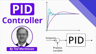
PID Control
🔒 Unlock Audio Lesson
Sign up and enroll to listen to this audio lesson
Lastly, let's put it all together with PID Control. Who can explain what PID stands for?
Proportional-Integral-Derivative!
Correct! PID combines all three controls to improve system response. The equation looks like this: \[ u(t) = K_p \cdot e(t) + K_i \int_0^t e(\tau) d\tau + K_d \frac{d}{dt} e(t) \]. Does anyone know an application for PID control?
Maybe in robotics for position control?
Exactly! It’s widely used in temperature control systems as well. And tuning these parameters is crucial for optimal performance. What are some methods we can use to tune PID controllers?
There’s the Ziegler-Nichols method, right?
Yes! Great recall. Understanding these control laws helps us design systems that fulfill performance requirements efficiently.
Practical Considerations for Implementing Control Laws
🔒 Unlock Audio Lesson
Sign up and enroll to listen to this audio lesson
Now that we’ve covered the control laws, let’s discuss practical considerations. What might we need to consider when implementing these controls in systems?
Sampling time is important, right?
Absolutely! Sampling time affects stability because we apply the control law at discrete times. What about computational needs?
We need real-time computing power for controllers!
Exactly! And we must also manage noise, perhaps through filtering. What are some differences between analog and digital controls?
Analog uses components like resistors and capacitors, while digital uses microcontrollers or PLCs, right?
Well done! These considerations are vital for successful control system implementation in diverse engineering applications.
Introduction & Overview
Read summaries of the section's main ideas at different levels of detail.
Quick Overview
Standard
The section explores fundamental control laws critical in engineering systems, including Proportional, Integral, Derivative, and PID controls. It presents their mathematical representations, implementation steps, and examples of applications, emphasizing their importance in achieving desired system performance. Limitations for each control type are also addressed.
Detailed
Implement Basic Control Laws in Practical Applications
This section discusses the core control laws used in practical engineering applications: Proportional (P), Integral (I), Derivative (D), and PID (Proportional-Integral-Derivative). Control laws are mathematical constructs that regulate system behavior through feedback mechanisms. The key points covered include:
Proportional Control (P)
- Definition: Proportional control adjusts the control input based on the immediate error.
- Mathematical Representation: The control input is calculated as \(u(t) = K_p imes e(t)\), where \(K_p\) is the proportional gain and \(e(t)\) is the error signal.
- Applications: Used in motor speed control and thermostats.
- Limitations: Causes steady-state error that cannot be eliminated.
Integral Control (I)
- Definition: This control type eliminates steady-state error by integrating past errors.
- Mathematical Representation: Captures accumulated error over time as \(u(t) = K_i \int_0^t e(\tau) d\tau\).
- Applications: Effective in temperature control and water level maintenance.
- Limitations: Susceptible to integral windup.
Derivative Control (D)
- Definition: Derivative control predicts future errors by focusing on the rate of change of error.
- Mathematical Representation: Given by \(u(t) = K_d \frac{d}{dt} e(t)\).
- Applications: Useful in motor control and damping vibrations.
- Limitations: Sensitive to noise in error signals.
PID Control
- Definition: This combines P, I, and D controls to enhance system performance.
- Mathematical Representation: \(u(t) = K_p \cdot e(t) + K_i \int_0^t e(\tau) d\tau + K_d \frac{d}{dt} e(t)\).
- Applications: Widely used in HVAC, motor speed control, and robotic positioning.
- Tuning Methods: Ziegler-Nichols, manual tuning, and software optimization are methods to adjust PID parameters for effective implementation.
Practical Considerations
- Sampling Time and Discretization: Emphasizes the importance of choosing appropriate sampling intervals to avoid instability.
- Computational Needs: Highlights the necessity for real-time computation capabilities in digital implementations.
- Noise and Disturbance Rejection: Discusses strategies like low-pass filtering to mitigate the effects of noise.
- Hardware Implementation: Outlines the differences between analog and digital control systems.
Understanding these control laws is crucial for designing and implementing reliable control systems across various engineering applications.
Youtube Videos
Audio Book
Dive deep into the subject with an immersive audiobook experience.
Introduction to Control Laws
Chapter 1 of 6
🔒 Unlock Audio Chapter
Sign up and enroll to access the full audio experience
Chapter Content
Control laws are the fundamental mathematical equations or algorithms that regulate system behavior. In engineering, the most common control laws used to implement control systems are Proportional (P), Integral (I), Derivative (D), and PID (Proportional-Integral-Derivative) control laws. These control laws are widely implemented in both hardware and software for a broad range of applications such as process control, robotics, automotive systems, electrical machines, and more.
Detailed Explanation
Control laws help engineers design systems that respond appropriately to changes in inputs or environments. They are mathematical formulas or algorithms that adjust the system's output to maintain a desired performance level. The four major types of control laws include Proportional (P), which adjusts the control signal based on the current error; Integral (I), which factors in past errors; Derivative (D), which predicts future errors based on their rate of change; and PID, which combines all three for comprehensive system control. These techniques can be applied in areas like industrial automation and robotics, influencing everyday technologies.
Examples & Analogies
Think of control laws like a car's driving system. When you press the gas pedal, the car accelerates based on how far you press it (Proportional). If the car's speed drops due to a hill, it adjusts for the cumulative loss of speed (Integral). If you're approaching a stop sign quickly, it monitors how fast you're slowing down to avoid overshooting (Derivative). Using a combination of these methods, the car maintains a smooth and safe ride.
Proportional Control (P)
Chapter 2 of 6
🔒 Unlock Audio Chapter
Sign up and enroll to access the full audio experience
Chapter Content
Proportional Control (P) is the simplest form of feedback control. It adjusts the control input based on the proportional error, i.e., the difference between the desired setpoint and the current output. Mathematical Representation: u(t)=Kp⋅e(t) where: ● u(t) is the control input. ● Kp is the proportional gain. ● e(t)=r(t)−y(t) is the error signal (difference between desired setpoint r(t) and the actual output y(t)).
Detailed Explanation
Proportional control uses the current error (the difference between the desired output and current output) to influence the control signal. The larger the error, the larger the control input; this is determined by the proportional gain, Kp. The goal is to reduce the error to a manageable level, but P control can't fully eliminate steady-state error, meaning that the system will stabilize near the setpoint but may not reach it exactly.
Examples & Analogies
Imagine using a dimmer switch to control the brightness of a light bulb. If the light is dimmer than you want, you turn the switch up proportionally to how dim it is. However, if you always set it just a bit lower than you want, the light will never be perfect, but it will get close to what you want depending on how much you turn the dial.
Integral Control (I)
Chapter 3 of 6
🔒 Unlock Audio Chapter
Sign up and enroll to access the full audio experience
Chapter Content
Integral Control (I) seeks to eliminate steady-state error by considering the accumulation of past errors. The integral action ensures that any persistent error over time results in a change in the control input, gradually driving the error to zero. Mathematical Representation: u(t)=Ki∫0te(τ)dτ where: ● u(t) is the control input. ● Ki is the integral gain. ● e(t) is the error signal.
Detailed Explanation
Integral control takes all the past errors into account and sums them over time. This continuous accumulation allows the control signal to adjust more significantly if there’s a consistent error. It drives the error towards zero, helping to eliminate any persistent offset that proportional control alone may not resolve. However, if the error stays large for too long, the accumulated controller input can become too high, resulting in instability (known as integral windup).
Examples & Analogies
Think of a bathtub filling with water. If you want the water level to be a specific height but it stays lower, the faucet will gradually increase the flow based on how long it has been below the desired level. If you forget to check it, the tub can overflow, just like an accumulated error can cause the controller to overshoot its target.
Derivative Control (D)
Chapter 4 of 6
🔒 Unlock Audio Chapter
Sign up and enroll to access the full audio experience
Chapter Content
Derivative Control (D) predicts the future error by considering the rate of change of the error. By responding to how fast the error is changing, derivative control helps to minimize overshoot and dampen oscillations in the system. Mathematical Representation: u(t)=Kd⋅ddte(t) where: ● u(t) is the control input. ● Kd is the derivative gain.
Detailed Explanation
Derivative control anticipates system behavior by measuring how quickly the error is changing over time. This is significant because it allows the control system to take proactive steps to adjust the output based on trends, such as rapidly increasing or decreasing errors. By incorporating this predictive aspect, derivative control helps reduce system oscillations and overshoot, leading to smoother control dynamics.
Examples & Analogies
Consider how a driver reacts while driving when approaching a curve. If they notice that they are speeding up or slowing down quickly in either direction, they will adjust their steering more cautiously, anticipating where they need to be. This forward-thinking approach helps avoid sharp turns or sudden stops, similar to how derivative control manages rapid changes in error.
PID Control
Chapter 5 of 6
🔒 Unlock Audio Chapter
Sign up and enroll to access the full audio experience
Chapter Content
PID Control combines Proportional (P), Integral (I), and Derivative (D) control laws to achieve robust control. The PID controller provides both immediate correction for error (P), correction for past errors (I), and predictive action to smooth out changes (D). This results in a system that minimizes error, eliminates steady-state error, and prevents overshoot. Mathematical Representation: u(t)=Kp⋅e(t)+Ki∫0te(τ)dτ+Kd⋅ddte(t)
Detailed Explanation
PID control integrates the strengths of all three control strategies to provide a comprehensive solution for regulating systems. The Proportional term addresses current errors, the Integral term accumulates past errors to prevent persistent offsets, and the Derivative term predicts future errors to facilitate smoother transitions. This holistic approach makes PID control particularly effective in maintaining stable and responsive system behavior across a variety of applications, from industrial processes to robotics.
Examples & Analogies
Imagine a chef trying to prepare a perfect dish. To get the flavor right, they taste the dish to adjust the seasoning (Proportional), remember how much seasoning was used in previous attempts to get a rich flavor (Integral), and watch not only the current taste but how rapidly the flavors are changing during cooking (Derivative). Using all these methods together, they consistently create perfectly balanced meals.
Practical Considerations for Implementing Control Laws
Chapter 6 of 6
🔒 Unlock Audio Chapter
Sign up and enroll to access the full audio experience
Chapter Content
- Sampling Time and Discretization: - In practical implementations, especially in digital systems, control laws are applied at discrete time intervals. - The control input is updated at each sampling time, so careful consideration of the sampling rate is important to avoid instability. 2. Computational Considerations: - PID and other control laws often require real-time computation, which may be performed on embedded systems (e.g., microcontrollers, FPGA, or PLC). - The computational power of the controller should be sufficient to compute the control law in real time.
Detailed Explanation
When implementing control laws, especially in digital systems, the timing of measurements and adjustments is crucial. Discrete sampling means that inputs and outputs are checked and updated at specific intervals, which must be selected wisely to ensure stability in the system. Additionally, the computations need to occur in real time, often requiring dedicated hardware capable of handling these calculations quickly and efficiently. Poor timing and inadequate computational resources can lead to system instability or failure, highlighting the importance of thoughtful implementation.
Examples & Analogies
Think of a sprinkler system that checks the soil moisture level every 10 seconds. If it checks too infrequently, the plants may wilt before the water is added. Conversely, if it checks too often without enough processing time, it may give erratic commands that lead to overwatering or underwatering. This shows how timing and computation matters greatly in automation systems.
Key Concepts
-
Proportional Control (P): Adjusts output based on current error.
-
Integral Control (I): Eliminates steady-state error by considering past errors.
-
Derivative Control (D): Predicts future error based on its rate of change.
-
PID Control: Combines P, I, and D controls for effective system management.
-
Tuning: The process of adjusting control parameters for optimal performance.
Examples & Applications
A thermostat using proportional control to regulate room temperature.
An oven employing integral control to maintain consistent cooking temperatures.
A robotic arm utilizing PID control to achieve precise movements.
Memory Aids
Interactive tools to help you remember key concepts
Rhymes
Proportional adjusts with speed,
Stories
Imagine a baker who adjusts the oven temperature (P) based on how far from the desired temp he is. If it’s too cool, he turns the heat up. But every time the thermometer indicates low temp for too long (I), he adds more heat! When he sees it's rising too quickly, he thinks ahead and lowers the heat (D) before it overshoots. This is like a PID controller baking perfectly!
Memory Tools
Remember 'PID' as 'Perfectly Integrated Dynamics' to recall the control components needed.
Acronyms
'PID' for Proportional, Integral, and Derivative—think of it as your guide to control!
Flash Cards
Glossary
- Control Laws
Mathematical equations or algorithms that regulate the behavior of a system.
- Proportional Control (P)
A control method that adjusts output proportionally to the error.
- Integral Control (I)
A control method that adjusts for past accumulated errors to eliminate steady-state error.
- Derivative Control (D)
A control method that anticipates future error by considering the rate of error change.
- PID Control
A control method combining Proportional, Integral, and Derivative controls for improved system performance.
- SteadyState Error
The persistent discrepancy between the desired output and the actual output of a control system.
- Integral Windup
A phenomenon where excessive accumulation of error leads to instability in control systems.
- Tuning
The process of adjusting controller parameters to optimize system performance.
- Sampling Time
The interval at which control actions are computed and applied in discrete systems.
- Noise
Unwanted disturbances that affect the performance of a control system.
Reference links
Supplementary resources to enhance your learning experience.