
Implementation Steps - 10.4.2
Enroll to start learning
You’ve not yet enrolled in this course. Please enroll for free to listen to audio lessons, classroom podcasts and take practice test.
Interactive Audio Lesson
Listen to a student-teacher conversation explaining the topic in a relatable way.
Introduction to Control Laws
🔒 Unlock Audio Lesson
Sign up and enroll to listen to this audio lesson

Today we'll discuss how to implement various control laws like Proportional, Integral, and Derivative in real systems. Can anyone tell me the difference between these control laws?

I think Proportional control just reacts to the error, but how is that different from Integral or Derivative?
Good question! Proportional control responds to the present error, while Integral control factors in past errors to eliminate steady-state errors. What about Derivative control?

Doesn’t Derivative control predict future errors based on the rate of change of the error?
Exactly! And when we combine these methods, we get PID control. Let’s look at the steps involved in implementing these controls.
Implementation Steps for Proportional Control
🔒 Unlock Audio Lesson
Sign up and enroll to listen to this audio lesson

Let's break down Proportional control. First, we define our desired setpoint. How might we gather the system's current output?

We could use sensors to measure the output!
Correct! After we have our output, we calculate the error. Can someone explain how that’s done?

We subtract the measured output from the desired setpoint!
Right. Next, we multiply this error by the proportional gain Kp to get our control input, which we then apply to the system. This is a straightforward approach, but what’s one limitation we must consider?
Proportional control can't eliminate steady-state error!
Exactly! Understanding this limitation helps us decide when to incorporate integral control next.
Understanding Integral Control
🔒 Unlock Audio Lesson
Sign up and enroll to listen to this audio lesson
Now, let’s explore Integral control. What is the first step we take when implementing it?
We measure the error between our setpoint and output!
Yes! Then we need to integrate this error over time. Why do you think this is important?
It helps us accumulate the error, so we can fix any steady-state issues?
Exactly! Now we can apply our integral gain Ki to compute the control input. What could be a drawback of this method?
Integral windup can happen if the error persists for too long.
That's an important point! We must be mindful of overshoot and stability in our systems.
Application of Derivative Control
🔒 Unlock Audio Lesson
Sign up and enroll to listen to this audio lesson
Let's now look at Derivative control. What’s our starting point?
We measure the current error and its rate of change!
Correct! Then we approximate that derivative, usually as the difference between current and previous errors. What’s the purpose of introducing the derivative term?
To dampen oscillations and help prevent overshoot!
Exactly! Although remember, Derivative control can be sensitive to noise. With that said, let's tie all this together with PID control.
Complete Steps for PID Control
🔒 Unlock Audio Lesson
Sign up and enroll to listen to this audio lesson
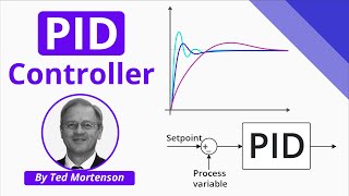
So, we’ve discussed Proportional, Integral, and Derivative controls separately. Why do you think we combine them in PID control?
To leverage the benefits of all three methods for better control!
Exactly! In PID, we measure the error and compute P, I, and D terms. Can someone summarize how we implement PID control?
We calculate each term and then sum them to get the control input to apply to the system!
Correct! PID tuning is also crucial. What methods can we use for that?
We can use the Ziegler-Nichols method or manually tune the parameters!
Great job, everyone! Remember that the implementation steps for control laws ensure effective regulation of dynamic systems.
Introduction & Overview
Read summaries of the section's main ideas at different levels of detail.
Quick Overview
Standard
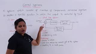
In this section, we delve into the systematic approach to implement Proportional (P), Integral (I), Derivative (D), and PID control laws. It discusses the necessary steps for measuring errors, calculating control inputs, and applying these inputs to regulate system behavior effectively.
Detailed
Implementation Steps
This section details the systematic steps required to implement various control laws including Proportional (P), Integral (I), Derivative (D), and PID in real-world applications. Each control law has distinct mechanisms and methodologies that guide their practical application.
Proportional Control (P) Implementation Steps:
- Set the Desired Setpoint (r(t)): Define the target value for the system.
- Measure Current Output (y(t)): Use sensors to measure the system's output.
- Calculate Error (e(t)): Determine the error as the difference between the setpoint and measured output: e(t) = r(t) - y(t).
- Compute Control Input (u(t)): Multiply the error by the proportional gain (Kp): u(t) = Kp * e(t).
- Apply Control Input: Adjust the system according to the computed control input, such as setting motor speed or controlling heating elements.
Integral Control (I) Implementation Steps:
- Measure Error (e(t)): As in P control, determine the difference between setpoint and output.
- Integrate the Error: Accumulate error over time, often implemented as a running total of previous errors.
- Compute Control Input (u(t)): Use the integral gain (Ki) with the total error: u(t) = Ki * ∫(0 to t) e(τ) dτ.
- Adjust the System: Control inputs adjust system operation based on accumulated error.
Derivative Control (D) Implementation Steps:
- Measure Current and Change in Error: Identify both the current error e(t) and its rate of change:
- Compute the derivative using past errors.
- Apply Derivative Gain: Calculate control input based on the change in error: u(t) = Kd * d/dt[e(t)].
- Implement the Control Input: Use the control input to manage rapid changes in system behavior.
PID Control Implementation Steps:
- Measure the Error: Identify the error as with earlier methods.
- Calculate P, I, and D Terms: Determine each component separately:
- Proportional: P = Kp * e(t)
- Integral: I = Ki * ∫(0 to t) e(τ) dτ
- Derivative: D = Kd * d/dt[e(t)]
- Combine the Control Terms: Sum these inputs for the overall control signal: u(t) = P + I + D.
- Apply the Control Input: Adjust the system accordingly to achieve desired outcomes.
These steps encapsulate the fundamental approach to implementing control theory in practice, crucial for achieving stability and performance in engineering systems.
Youtube Videos
Audio Book
Dive deep into the subject with an immersive audiobook experience.
Step 1: Measure the Error
Chapter 1 of 4
🔒 Unlock Audio Chapter
Sign up and enroll to access the full audio experience
Chapter Content
- Measure the error e(t)e(t) and its rate of change ddte(t) (t).
Detailed Explanation
The first step in implementing derivative control is to measure the current error and how quickly that error is changing. The error is defined as the difference between the desired output and the actual output of the system. This measurement gives us an idea of how far off the system is from where we want it to be. Additionally, we also need to calculate the rate at which this error is changing, which helps us predict if it will increase or decrease in the future.
Examples & Analogies
Imagine you're trying to catch a ball thrown at you. When you notice the ball (error), you also observe how fast it's approaching (rate of change of error). By measuring both, you can better position yourself to catch it successfully.
Step 2: Calculate the Derivative of the Error
Chapter 2 of 4
🔒 Unlock Audio Chapter
Sign up and enroll to access the full audio experience
Chapter Content
- Calculate the derivative of the error, often approximated in discrete systems as the difference between current and previous errors.
Detailed Explanation
In this step, we need to calculate the derivative of the error. This can be done by taking the difference between the current error and the error from the previous time step. This gives us the rate of change of the error, which is crucial for understanding how fast the error is increasing or decreasing. In practical digital systems, this method approximates the mathematical derivative to make real-time calculations possible.
Examples & Analogies
Think of it like riding a bicycle downhill. If you notice you're going faster than before, you're calculating how your speed is increasing (the derivative of speed). The more rapidly you're accelerating downhill, the more corrective action you may need to take to steer.
Step 3: Compute the Control Input
Chapter 3 of 4
🔒 Unlock Audio Chapter
Sign up and enroll to access the full audio experience
Chapter Content
- Multiply the derivative by the gain KdK_d to compute the control input.
Detailed Explanation
Once we have the derivative of the error, the next step is to multiply this value by the derivative gain (Kd). This gain determines how sensitive our control system will be to changes in the error. The result is the control input, which indicates how much correction is needed in the system to counteract the rate of change of the error. This control input will help moderate the system's response, smoothing out any rapid changes.
Examples & Analogies
Imagine using the brakes on a car. The harder you press (which can be likened to the gain Kd), the quicker the car slows down in response to how fast you're approaching a stoplight (the error). Adjusting your braking force precisely helps you slow down without skidding.
Step 4: Apply the Control Input
Chapter 4 of 4
🔒 Unlock Audio Chapter
Sign up and enroll to access the full audio experience
Chapter Content
- Apply the control input to the system to counteract rapid changes in error.
Detailed Explanation
The final step in the implementation of derivative control is applying the calculated control input to the system. This adjustment helps the system counteract any rapid changes in error that were predicted based on the calculated derivative. By applying this corrective action, the system can become more stable and respond appropriately to variations, thereby minimizing overshoot and oscillations.
Examples & Analogies
Think of this as adjusting the throttle on your motorcycle when you feel it accelerating too quickly. By smoothly easing off on the throttle (applying control), you manage your speed, preventing sudden jerks that might throw you off balance.
Key Concepts
-
Proportional Control: Adjusts the control input based on the present error.
-
Integral Control: Accumulates past errors to eliminate steady-state error.
-
Derivative Control: Responds to the rate of error change to minimize overshoot.
-
PID Control: Combines P, I, and D actions to provide robust control.
Examples & Applications
A thermostat maintains temperature by adjusting the heating element based on the temperature error.
In industrial automation, PID controllers manage motor speeds, providing smooth and accurate performance.
Memory Aids
Interactive tools to help you remember key concepts
Rhymes
For control that's smart, use P, I, D; stabilize the system, let your goals be freed.
Stories
Once upon a time, a factory tried to regulate its machines. The Proportional knight would react quickly to errors. The wise Integral king would remember past mistakes, while the Derivative mage predicted future woes. Together, they ruled in harmony as PID.
Memory Tools
Remember 'PID' - P is for Present error, I is for Integrating past actions, and D is for Deriving future strategies.
Acronyms
PID
- Proportional
- Integral
- Derivative.
Flash Cards
Glossary
- Control Law
A mathematical equation or algorithm that dictates the behavior of a control system.
- Proportional Control (P)
A control strategy that adjusts control input based on the proportional error.
- Integral Control (I)
A control strategy that eliminates steady-state error by considering the accumulation of past errors.
- Derivative Control (D)
A control strategy that predicts future error by considering the rate of change of the error.
- PID Control
A control strategy that combines Proportional, Integral, and Derivative controls for robust system regulation.
Reference links
Supplementary resources to enhance your learning experience.