
Concentration Distribution in an Ideal Plume
Enroll to start learning
You’ve not yet enrolled in this course. Please enroll for free to listen to audio lessons, classroom podcasts and take practice test.
Interactive Audio Lesson
Listen to a student-teacher conversation explaining the topic in a relatable way.
Introduction to Steady State Assumptions
🔒 Unlock Audio Lesson
Sign up and enroll to listen to this audio lesson

Today, we will explore the concept of steady-state assumptions in concentration distribution. Can anyone explain what we mean by steady state?

It means that the concentration at a specific point doesn’t change over time.
Exactly! When we say that concentration remains constant over time, we're simplifying our calculations since we can assume emissions are steady as well. Remember this acronym: 'SEC' for 'Steady Emission Concentrations'.

How does this relate to our environment? Isn’t everything constantly changing?
Great point! Although the assumption simplifies our model, in reality, environmental factors continuously impact emissions and concentrations. That’s why we often work with average values and variations.

So, can we assume that conditions are ideal in a real-world scenario?
Not really. While this model provides a baseline, real applications often require adjustments due to changing conditions. Let's summarize: we apply the SEC model under idealized conditions but always acknowledge the fluctuations in reality.
Mathematical Modeling of Dispersion
🔒 Unlock Audio Lesson
Sign up and enroll to listen to this audio lesson

Now, let’s look at how we mathematically model dispersion in three dimensions. Who can remind us of the terms involved?

Delta Na by delta y and delta Na by delta z?
Correct! By considering dispersion across x, y, and z axes, we can create a more comprehensive picture of the plume. Remember: 'D3' stands for 'Dimension Three Modeling'.
What does the term Q represent in this context?
Q refers to the rate of pollutant release, integrating across z-axis limits. So, integrating concentration over the entire volume gives us valuable insights.
How do we ensure accuracy with these calculations?
Accuracy is paramount! We need to understand the constants we incorporate and establish proper boundary conditions to ensure we effectively capture plume behavior.
Understanding Gaussian Distribution
🔒 Unlock Audio Lesson
Sign up and enroll to listen to this audio lesson
Moving on, let’s connect our discussions to Gaussian distributions. Why do we consider Gaussian models for plume concentration?
Because they show how pollutants typically spread out in a bell-shaped curve?
Exactly! Concentrations peak at a certain point and taper off. We can remember this idea with the acronym 'BIFT' for 'Bell-Inverted Fluctuating Totals'.
So, is the concentration always highest at the center of this ideal plume?
Yes, it usually is! The position of this peak depends directly on the plume's characteristics and environmental conditions.
Why do we analyze the spread of this concentration?
Analyzing the spread helps us understand how to manage pollutant impact effectively. Always remember: Concentration and its spread matter for public health and environmental protection!
Real-world Implications of Ideal Models
🔒 Unlock Audio Lesson
Sign up and enroll to listen to this audio lesson
Finally, let's discuss the practical implications of what we've learned today. Can someone give an example of this model in real life?
Like how we predict pollution levels in cities?
Exactly! However, remember that these models can oversimplify reality. We must account for variations, so always apply caution when interpreting results. Use the mnemonic 'PREDICT' which stands for 'Pollution Realities in Emission Dispersal & Interactions Complexity'.
How can we adjust our models to enhance their accuracy in practical scenarios?
By incorporating real-time data, adjusting parameters based on observed variations, and continuously validating our models. This leads to more reliable predictions!
Got it! It’s about balancing the ideal with the real.
Precisely! Always remember that understanding both sides enhances our analysis and decision-making.
Introduction & Overview
Read summaries of the section's main ideas at different levels of detail.
Quick Overview
Standard
This section explores the fundamentals of concentration distribution in an ideal plume, highlighting the use of Gaussian dispersion models under steady state assumptions. It elaborates on the mathematical formulation of plume dispersion in three dimensions, boundary conditions, and the implications of environmental factors on concentration averages.
Detailed
Concentration Distribution in an Ideal Plume
This section elaborates on the mathematical modeling of pollutant dispersion in an ideal plume using Gaussian distribution principles. Initially, it addresses the steady-state assumption, which holds that concentrations do not change over time at fixed locations, thus simplifying the analysis. Under steady state conditions, parameters such as emission rates must remain constant.
The section progresses to define how the dispersion occurs along three spatial dimensions—x, y, and z. The teacher discusses how the general solution incorporates mass conservation principles and integrates these across the plume volume.
A significant point of focus is how the Gaussian distribution model relates to concentration dispersal in plumes. This entails plotting concentration against distance to illustrate how the highest concentrations occur at specific points in relation to y and z axes, forming ideal bell-shaped curves. The teacher notes that while these curves are idealized, they serve as essential approximations in understanding pollutant behavior.
The section concludes with transformations of the Gaussian equation that help tailor the model to various emission scenarios, ultimately stressing the variable nature of wind direction and its influence on concentration distribution.
Youtube Videos

![[ADI] PLUME BEHAVIOUR (ENVIRONMENT ENGINEERING) EXPLAINED (CE)!!! In Hindi](https://img.youtube.com/vi/pUaqNCqAgFc/mqdefault.jpg)


Audio Book
Dive deep into the subject with an immersive audiobook experience.
Assumptions of Steady State
Chapter 1 of 4
🔒 Unlock Audio Chapter
Sign up and enroll to access the full audio experience
Chapter Content
Now here we make two assumptions, one is a steady state assumption you don’t have to do this but for that Gaussian dispersion model that we generally present we use the steady state assumptions where we say C(x,y,z,t) = 0, which means that at any point in time the concentration is the same, at any location you measure it concentration will not change with time. It will be different with space but it will not change with time.
Detailed Explanation
In this section, we first discuss a crucial assumption known as the steady state assumption in environmental dispersion modeling. Steady state means that the concentration of a pollutant at any given location does not change over time, although it can vary from place to place. For this assumption to hold true, the emission of pollutants must be constant, and external conditions affecting concentration must not change. If any parameter in the model changes over time, this assumption no longer applies.
Examples & Analogies
Think of a bathtub that is constantly filled with water at the same rate while the drain remains unblocked. The water level remains constant over time, similar to how concentrations remain steady in a steady state assumption. However, if someone unexpectedly changes the flow rate or opens the drain, the water level will start changing, just like the concentration would if any of the underlying conditions changed.
Simplifying the Dispersion Equation
Chapter 2 of 4
🔒 Unlock Audio Chapter
Sign up and enroll to access the full audio experience
Chapter Content
These second thing that we do is since we already have u_x bulk flowing in the x direction. We neglect this dx term, so this entire thing reduces to this simple equation.
Detailed Explanation
In modeling pollutant dispersion, we often simplify equations to focus on the most significant factors. Here, we note that there is an existing flow of pollutants in the x-direction (u_x). Because this flow direction is already accounted for, we can simplify our equation by neglecting the dx term related to this directional flow. This process allows us to concentrate on the essential aspects of dispersion, particularly how pollutants spread in the y and z directions.
Examples & Analogies
Imagine driving a car straight down a highway. If you want to analyze how much the car sways from side to side, it makes sense to focus on that side-to-side motion rather than the straight path ahead. Similarly, in our model, we focus on how pollutants disperse upwards and sideways rather than the established flow direction.
General Solution for Plume Concentration
Chapter 3 of 4
🔒 Unlock Audio Chapter
Sign up and enroll to access the full audio experience
Chapter Content
Normally when you say boundary condition will say x equals to x1 value of rho_A is this much or something happens to flux, there is a wall boundary condition and all that. We fix the values or we give some indication as to what it is.
Detailed Explanation
In developing a theoretical model, it is essential to set boundary conditions, which are constraints that define how the system behaves in specific situations. In essence, we specify parameters such as pollutant concentration at certain points or conditions related to walls or barriers. By establishing these conditions, we can solve for the overall concentration throughout the plume. By integrating these conditions mathematically, we approach a general solution that encompasses various scenarios.
Examples & Analogies
Consider a swimming pool where you determine the maximum height of the water when filling it up. If you know the pool's dimensions and how much water you’re adding per minute, you can predict when the pool will be full or how quickly it will reach the overflow. Similarly, in our model, setting boundary conditions helps us predict pollutant concentration in a plume.
Gaussia Distribution and Its Comparison
Chapter 4 of 4
🔒 Unlock Audio Chapter
Sign up and enroll to access the full audio experience
Chapter Content
So, where do you find the highest concentration? Where will you find it? So, we look at an ideal plume. An ideal plume is nicely going in this cone kind of fashion. The cross-section looks like an ellipse or even a circle.
Detailed Explanation
In an ideal scenario, pollutants disperse from a source in a structured manner, forming a plume that resembles a cone or cylinder. The distribution of concentration within this plume reaches its peak at the center and diminishes to zero at the edges. This pattern allows us to visualize where the highest concentrations of pollutants will occur, helping predict potential impact zones based on their spread and concentration. Understanding this Gaussian-like distribution is key to environmental assessments.
Examples & Analogies
Think of a spray bottle. When you spray water, the droplets form a cone shape as they disperse. If you measure the concentration of water droplets closer to the nozzle, the amount is highest there and decreases as the distance from the nozzle increases. This concept of concentration distribution in a plume is similar: the maximum concentration is at the center and spreads out, just like how the water droplets disperse from the spray.
Key Concepts
-
Steady State: The assumption that the concentration at any point does not change with time.
-
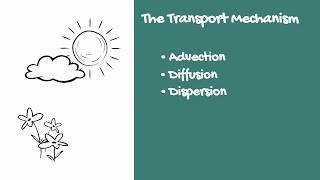
Dispersion: The way pollutants spread through the environment, modeled in three dimensions.
-
Gaussian Distribution: A statistical representation of pollutant concentrations that often approximates how emissions disperse.
Examples & Applications
Example of a power plant where emissions create a plume dispersing pollutants into the surrounding atmosphere.
Case of urban traffic where vehicle emissions disperse pollutants in a Gaussian pattern influenced by wind.
Memory Aids
Interactive tools to help you remember key concepts
Rhymes
Pollutants disperse high and wide, in Gaussian curves, they often glide.
Stories
Imagine a factory releasing smoke; it rises swiftly and spreads like a big, fluffy cloud, eventually fading away, following the Gaussian path of highest concentration at its center.
Memory Tools
Remember 'BIFT' - Bell-Inverted Fluctuating Totals, to signify Gaussian curves in concentration distribution.
Acronyms
Use 'SEC'—Steady Emission Concentrations to remind you of steady state assumptions in pollution modeling.
Flash Cards
Glossary
- Steady State
A condition in which the concentration of a pollutant remains constant over time at a fixed location.
- Gaussian Distribution
A statistical distribution that represents data with a bell-shaped curve, commonly used to model concentrations of pollutants in a plume.
- Dispersion
The spread of pollutants in the environment, which can occur in multiple dimensions.
- Boundary Condition
Constraints set on the variables of a mathematical model to match physical situations.
- Plume
The aerial column of pollutants released from a source into the environment.
Reference links
Supplementary resources to enhance your learning experience.