
Gaussian Distribution
Enroll to start learning
You’ve not yet enrolled in this course. Please enroll for free to listen to audio lessons, classroom podcasts and take practice test.
Interactive Audio Lesson
Listen to a student-teacher conversation explaining the topic in a relatable way.
Understanding Steady State Assumptions
🔒 Unlock Audio Lesson
Sign up and enroll to listen to this audio lesson

Today, we will explore the idea of steady state assumptions related to the Gaussian distribution. Can someone tell me what 'steady state' means in this context?

Does it mean that the concentration of pollutants does not change over time?
Exactly! In a steady state, the concentration at each location remains constant over time, though it does vary from place to place. This is critical for our equations to work. What happens if something changes over time?

Then we can no longer assume steady state?
Correct! If emission rates or environmental conditions fluctuate, the model no longer holds. Remember—steady state = constant concentration in variable locations. A good mnemonic for this is 'Stay Steady, Stay Constant'!
Gaussian Dispersion Model
🔒 Unlock Audio Lesson
Sign up and enroll to listen to this audio lesson

Now, let's look at how we derive the Gaussian dispersion model mathematically. Who remembers the equation we use?

Is it the one that looks like a bell curve?
Yes! The Gaussian equation can be represented as a normal distribution curve. The width of this curve is determined by the standard deviation. Who can explain what affects the standard deviation in our model?

I think it's related to how spread out the pollutants are, right?
Exactly! The greater the spread, the lower the peak concentration, as conservation laws dictate. That’s a critical insight!
Boundary Conditions in Dispersion
🔒 Unlock Audio Lesson
Sign up and enroll to listen to this audio lesson
Last time, we briefly touched on boundary conditions. Can anyone summarize what they are?
They are the constraints and limits on where the pollutant can spread?
Exactly! For example, a plume can expand infinitely in the y-direction and is limited in the z-direction due to the ground. Understanding these boundaries is crucial for accurately modeling dispersion.
So, applies to how we integrate our equations?
Exactly! Integration over these bounds helps us to determine total mass flow. Remember, 'Boundaries Confine Flow'!
Real-world Applications of Gaussian Distribution
🔒 Unlock Audio Lesson
Sign up and enroll to listen to this audio lesson
How do you think understanding the Gaussian distribution aids in environmental management?
It helps predict where pollutants will spread and how concentrated they'll be.
Absolutely! By applying this model, environmental scientists can set regulations to manage emissions effectively. It’s about mitigating impact on public health. A cautionary phrase: 'Spread Wisely, Pollute Cautiously!'
Introduction & Overview
Read summaries of the section's main ideas at different levels of detail.
Quick Overview
Standard
The section outlines the Gaussian distribution model, focusing on the steady state assumptions that lead to a simplified equation for pollutant dispersion in three dimensions. It covers essential concepts like boundary conditions and concentration distribution, illustrating how these factors impact the pollutant's behavior in the environment.
Detailed
The section elaborates on the Gaussian distribution model as it pertains to pollutant dispersion, emphasizing the steady state assumption where concentration remains constant over time but varies with location. This assumption allows simplification of complex equations governing pollutant behavior. The discussion extends to various boundary conditions relevant to dispersion, integrating mass conservation principles into the equation governing pollutant flow. The Gaussian distribution is presented as an idealized bell curve representing the concentration of pollutants. Understanding this model is crucial for environmental management and regulatory standards.
Youtube Videos


Audio Book
Dive deep into the subject with an immersive audiobook experience.
Understanding Steady-State Assumption
Chapter 1 of 5
🔒 Unlock Audio Chapter
Sign up and enroll to access the full audio experience
Chapter Content
Now here we make two assumptions, one is a steady state assumption you don’t have to do this but for that Gaussian dispersion model that we generally present we use the steady state assumptions where we say &)!" = 0, which means that at any point in time the concentration is &* the same, at any location you measure it concentration will not change with time. It will be different with space but it will not change with time.
Detailed Explanation
In this chunk, we discuss the steady-state assumption used in modeling Gaussian dispersion. This assumption states that at any specific location, the concentration of a substance remains constant over time, meaning any variations occur only with changes in space. For instance, if we measure air pollution at a certain spot, the concentration we find today will be the same tomorrow, assuming no new emissions. However, it will differ from concentrations at other locations.
Examples & Analogies
Imagine a candle burning steadily in a room. The smell (or concentration of the scent) near the candle remains constant over time, but as you move further away from the candle, the scent lessens. This reflects how the concentration can vary with distance (space) but remains constant at a given spot over time, similar to our steady-state assumption.
Mass Conservation in Gaussian Dispersion
Chapter 2 of 5
🔒 Unlock Audio Chapter
Sign up and enroll to access the full audio experience
Chapter Content
So we are saying Q is the rate of pollutant release equals u multiplied by dy and dx...
Detailed Explanation
This chunk emphasizes the principle of mass conservation within the Gaussian dispersion model. Q, representing the rate of pollutant release, is calculated from the product of the wind speed (u) and the dimensions of the dispersion in the y (dy) and x (dx) directions. The equation suggests that the total mass of the pollutant in the plume remains constant over time, conserving mass at all points within the dispersion's limits.
Examples & Analogies
Think about water flowing through a hose. The rate at which water exits the hose (analogous to Q) must equal the amount of water being pushed through the hose by the pressure inside. If we slightly reduce the diameter of the hose (similar to incorporating dy and dx), the water spreads out but conserves the total amount flowing out.
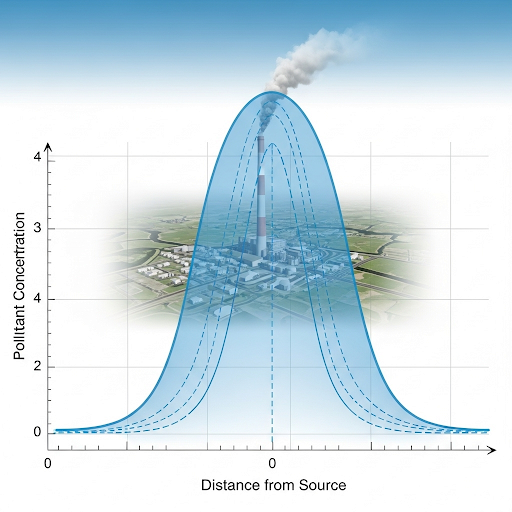
Introduction to Gaussian Distribution
Chapter 3 of 5
🔒 Unlock Audio Chapter
Sign up and enroll to access the full audio experience
Chapter Content
Now, the general solution for this, this is an equation there are solutions are already there...very similar to another equation which is called as a Gaussian distribution or a normal distribution.
Detailed Explanation
In this section, we introduce the Gaussian distribution in relation to the Gaussian dispersion model. The Gaussian distribution describes how concentrations of pollutants can be expected to vary in space, depicting a bell-shaped curve. Depending on the variability (or standard deviation) of the concentration spread, this curve can either be narrow (high concentration) or wide (low concentration).
Examples & Analogies
Imagine dropping a pebble into a calm pond. The ripples that spread out create a bell-shaped pattern where the peak concentration of water movement is right at the point of entry, tapering off as you move further away. This visually represents how pollutants disperse from a source in a Gaussian model.
Ideal Plume Characteristics
Chapter 4 of 5
🔒 Unlock Audio Chapter
Sign up and enroll to access the full audio experience
Chapter Content
Where do you find the highest concentration? Where will you find it? So for which we look at an ideal plume...
Detailed Explanation
This chunk describes the characteristics of an ideal plume, including how pollutant concentration is highest at the center of the plume. The concentration distribution is often visualized as an ellipse or circle, where the concentration is highest at certain coordinates. External factors, such as wind direction and speed, dictate how the plume spreads.
Examples & Analogies
Imagine a blender mixing a smoothie. The center of the blender (the ideal plume's peak concentration) will have a richer concentration of ingredients, while the further you go from the center to the edges, the less intense the flavor becomes, illustrating how concentration disperses.
Transforming the Gaussian Equation
Chapter 5 of 5
🔒 Unlock Audio Chapter
Sign up and enroll to access the full audio experience
Chapter Content
Now to make it look like this you have to do some transformation so one of the transformation is this one this one we do sigma y and sigma z into 2 Dyx divided by ux and so on...
Detailed Explanation
In this chunk, we explore transformations to the Gaussian distribution equation, adjusting parameters to fit observed data. These transformations help define where the highest concentration occurs concerning the source of pollution, aiding in making accurate predictions about pollutant behavior.
Examples & Analogies
Consider using a map to find directions. Sometimes, you must adjust your starting point or the route to reach your destination efficiently. Similarly, transforming the Gaussian equation helps us accurately predict how pollutants disperse based on different starting conditions.
Key Concepts
-
Steady state: Concentration remains constant in time.
-
Gaussian distribution: A bell-shaped curve representing concentration values.
-
Boundary conditions: Limits affecting pollutant dispersion.
Examples & Applications
Air quality assessments use Gaussian distribution to predict pollutant concentrations in urban areas.
Gaussian dispersion model helps regulatory agencies design effective pollution control strategies.
Memory Aids
Interactive tools to help you remember key concepts
Rhymes
In a Gaussian arc, pollutants make their mark; steady in their race, with boundaries to trace.
Stories
Imagine a river of pollution flowing smoothly; as it reaches boundaries, it spreads out and changes shape, just like the Gaussian curve.
Memory Tools
G-B-S: Gaussian for Bell-shaped, Steady for time constant.
Acronyms
GEM
Gaussian
Emission
Model—components of dispersion modeling.
Flash Cards
Glossary
- Gaussian Distribution
A statistical distribution characterized by a symmetric bell-shaped curve described by its mean and standard deviation.
- Steady State
A condition where the concentration of pollutants does not change over time at a specific location.
- Boundary Conditions
Constraints that define the limits within which the pollutant dispersion model applies.
- Concentration
The amount of a substance (pollutant) present in a specific volume.
- Dispersion
The process of pollutants spreading out from a source, influenced by various environmental factors.
Reference links
Supplementary resources to enhance your learning experience.