
General Solution
Enroll to start learning
You’ve not yet enrolled in this course. Please enroll for free to listen to audio lessons, classroom podcasts and take practice test.
Interactive Audio Lesson
Listen to a student-teacher conversation explaining the topic in a relatable way.
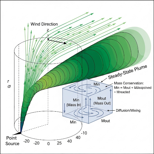
Steady-State Assumptions
🔒 Unlock Audio Lesson
Sign up and enroll to listen to this audio lesson

Today, let's begin with the steady-state assumption in our dispersion model. Can anyone tell me what this means?

Does it mean that the concentration of pollutants doesn’t change over time at a particular location?
Exactly! The concentration might vary from one location to another, but at any specific point, it remains constant. This simplifies our calculations. We call it a steady-state assumption. Remember the acronym 'SCA' for Steady, Constant, and Assumed.

What happens if things change over time?
Good question! If parameters change, then we cannot use this assumption, and we'd have to consider more complex models.
To summarize, in a steady-state assumption, pollutant concentrations remain constant at any point but can differ spatially.
Dispersion in Three Dimensions
🔒 Unlock Audio Lesson
Sign up and enroll to listen to this audio lesson

Next, let’s dive into how we model dispersion across three dimensions. Who can explain why this matters?

Dispersion affects how and where pollutants spread in the environment, right?
Exactly! We express pollutants' movement mathematically in terms of three dimensions: x, y, and z. To ensure mass is conserved, we use principles of physics in our equations.
What do we actually mean by mass conservation in this context?
Mass conservation means that the total mass entering a volume must equal the mass leaving it, plus any changes within.
In summary, dispersion in three dimensions allows us to visualize and calculate how pollutants spread, influenced heavily by mass conservation.
Gaussian Distribution Relation
🔒 Unlock Audio Lesson
Sign up and enroll to listen to this audio lesson
Now, let's connect our model to Gaussian distribution. Why do we model pollutant dispersion in this way, you think?

Because many natural processes approximate a Gaussian distribution, like how particles spread out in the atmosphere?
Exactly, well said! The Gaussian distribution helps us predict where the highest pollutant concentrations usually occur.
Can we visualize this?
Certainly! Picture the concentration peak as the center of a bell curve — this is exactly how pollutants behave in an ideal situation. Always remember: 'higher distribution means lower concentration'.
To summarize, the Gaussian distribution offers a powerful tool for understanding and predicting pollutant dispersion.
Introduction & Overview
Read summaries of the section's main ideas at different levels of detail.
Quick Overview
Standard
In this section, we explore the general solution for dispersion equations of pollutants in a 3D space, emphasizing steady-state assumptions, mass conservation within a plume, and how these lead to Gaussian distribution models, ultimately helping to understand pollutant concentration distribution.
Detailed
General Solution
This section focuses on the derivation and explanation of the general solution for dispersion equations used to model pollutant distributions in a three-dimensional space. The discussion emphasizes two fundamental assumptions:
- Steady-state assumption: This means that the concentration of pollutants remains constant over time at any specific point in space despite variations across locations. It assumes that the emission rate and environmental conditions are also constant.
-
Mass conservation: The equation governing pollutant dispersion in the plume is derived using the principles of mass conservation, indicating that the total mass present in the plume can be expressed in terms of the emission rates and dispersion parameters.
The general solution incorporates these principles and reduces to simpler forms when neglecting certain terms. The derived equation models how pollutants disperse in three dimensions, notably under Gaussian distribution assumptions, allowing for practical applications in environmental science.
Youtube Videos


Audio Book
Dive deep into the subject with an immersive audiobook experience.
Assumptions for the Gaussian Dispersion Model
Chapter 1 of 5
🔒 Unlock Audio Chapter
Sign up and enroll to access the full audio experience
Chapter Content
Now here we make two assumptions, one is a steady state assumption...we make our decisions based on it.
Detailed Explanation
In this chunk, we discuss two key assumptions underlying the Gaussian dispersion model. The first is the 'steady state assumption', which means that the concentration of pollutants at any fixed location does not change over time. While it may vary based on location, it remains constant when measured at the same spot. This is critical because it implies that the emission rate of pollutants and their characteristics must also stay constant over time. If any parameter changes, the steady state assumption is no longer valid. The second point emphasizes the importance of statistical analysis, as environmental conditions are never perfectly constant. Therefore, average values are used to make predictions and decisions.
Examples & Analogies
Imagine a water fountain that spills water continuously without stopping. If you were to measure the amount of water at a certain point directly in front of the fountain, you would see that it does not change over time; that's like a steady state assumption. However, if there is a sudden change like the water fountain getting turned off or on, your measurement would change, invalidating your initial assumption.
The Simplification of the General Solution
Chapter 2 of 5
🔒 Unlock Audio Chapter
Sign up and enroll to access the full audio experience
Chapter Content
Weneglect this dx term, so this entire thing reduces to this simple equation...
Detailed Explanation
In this part, the speaker simplifies the model by neglecting certain variables—specifically the 'dx term', which represents changes in the x-direction. As a result, the model condenses into a more manageable form, allowing for easier calculations and understanding of the pollutant's dispersion in the air across three dimensions—x, y, and z.
Examples & Analogies
Think of simplifying a complex recipe by removing unnecessary ingredients. If a recipe has multiple steps and ingredients that aren't essential, you can simplify it to focus on the core flavors. In the context of air pollution modeling, ignoring certain factors helps clarify the situation.
General Solution and Boundary Conditions
Chapter 3 of 5
🔒 Unlock Audio Chapter
Sign up and enroll to access the full audio experience
Chapter Content
The general solution for this... the entire volume is coming from the source...
Detailed Explanation
Here, the general solution of the Gaussian model is presented. The speaker explains the importance of boundary conditions which set the limits within which the solution applies. For example, the boundaries of the plume concerning the three dimensions (x, y, and z) can be defined: the plume extends infinitely in the y-direction, but has limits in the z-direction due to ground level constraints. Understanding these boundaries helps determine how pollutants disperse from a given source.
Examples & Analogies
Imagine you pour a drop of food coloring into water in a tall glass. The color spreads out perfectly, but the height of the water provides a limit on how high the color can rise. In this analogy, the boundaries of the glass represent the z-direction limits, while the freely spreading color illustrates the dispersion in the y-direction.
Transformations and Idealized Plume Geometry
Chapter 4 of 5
🔒 Unlock Audio Chapter
Sign up and enroll to access the full audio experience
Chapter Content
Now, the Gaussian dispersion model...you have to do some transformation...
Detailed Explanation
This section discusses the transformation needed to relate the Gaussian dispersion model with real-world observations. It introduces a Gaussian distribution equation and accommodates environmental variables like wind direction and source shape. The idealized plume follows a bell-shaped curve which denotes pollutant concentration over time. These transformations allow the model to accurately represent pollutant behavior in various scenarios.
Examples & Analogies
Imagine throwing a pebble into a calm pond. The ripples created represent the dispersion of pollutants. The way the ripples spread out can be likened to adjusting parameters in our equations to account for environmental conditions. If you use a heavier stone (more pollutants), the ripples will behave differently than with a lighter one, just as the plume's concentration changes with different emission sources.
Understanding Concentration Distribution
Chapter 5 of 5
🔒 Unlock Audio Chapter
Sign up and enroll to access the full audio experience
Chapter Content
So, where do you find the highest concentration?... this does not usually happen a lot of times.
Detailed Explanation
This chunk elaborates on the characteristics of concentration distribution within pollutants in the plume. It discusses how concentration typically reaches its maximum at a specific point within the plume and illustrates the balance between concentration and spread. While an idealized Gaussian distribution is visually represented as a symmetric bell curve, real-world data may show deviations from this shape, leading to skewed results. However, the bell-curve model serves as a valuable approximation for understanding pollution distribution.
Examples & Analogies
Consider a crowded concert. The area right in front of the stage has the highest concentration of people, akin to the point of highest pollutant concentration in the model. As you move away from the stage, the number of people (or concentration) diminishes. In reality, people might cluster in uneven ways, just like pollutant concentrations can vary.
Key Concepts
-
Steady-state assumption: A fundamental underpinning in dispersion modeling.
-
Mass conservation: The principle ensuring mass is accounted for during dispersion.
-
Dispersion mechanics: Understanding how pollutants spread across different axes.
-
Gaussian distribution: A relevant statistical model for visualizing pollutant concentration.
Examples & Applications
When modeling the concentration of pollutants emitted from a factory, the steady-state assumption can simplify calculations by considering fixed rates over time.
Using Gaussian distribution, we can predict the highest concentration of pollutants will occur directly downwind from a source.
Memory Aids
Interactive tools to help you remember key concepts
Rhymes
In steady-state, the pollution stays, a constant sight through all our days.
Stories
Imagine a well-controlled factory emitting smoke; it keeps ambient pollution steady over time, letting us measure accurately.
Memory Tools
Remember 'SPM': Steady-state, Peak concentrations, Mass conservation!
Acronyms
Use 'GDS' for Gaussian Distribution's Significance.
Flash Cards
Glossary
- SteadyState Assumption
The assumption that pollutant concentration remains constant over time at any specific location.
- Mass Conservation
A principle stating that the total mass within a closed system remains constant over time.
- Dispersion
The process by which pollutants spread through the environment, typically represented in three dimensions.
- Gaussian Distribution
A statistical distribution often used to describe real-valued random variables with a symmetrically bell-shaped curve.
- Plume
A mass of airborne contaminants expelled from a source, dispersing through the atmosphere.
Reference links
Supplementary resources to enhance your learning experience.