
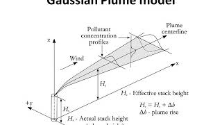
Final Form of the Gaussian Dispersion Model
Enroll to start learning
You’ve not yet enrolled in this course. Please enroll for free to listen to audio lessons, classroom podcasts and take practice test.
Interactive Audio Lesson
Listen to a student-teacher conversation explaining the topic in a relatable way.
Introduction to the Gaussian Dispersion Model
🔒 Unlock Audio Lesson
Sign up and enroll to listen to this audio lesson

Welcome to our class on Gaussian dispersion. Today, we will focus on the model's final form. To start, let's discuss the steady-state assumption. Who can tell me what it means?

Does it mean that the concentration stays constant over time?
Exactly! The steady-state assumption implies that concentration changes only with position, not time. This means emissions must remain constant during the observation. Let's remember this with the acronym 'CPT' - Constant Pollution Trickle.

So, if variables change with time, we can't use this model?
That's correct! If conditions vary, the steady-state assumption wouldn't hold. Now, let's dive into the three-dimensional representation.
Mathematical Representation
🔒 Unlock Audio Lesson
Sign up and enroll to listen to this audio lesson

Now, we simplify the dispersion equation by assuming bulk flow. Can anyone explain what we neglect to get to simpler equations?

We neglect the dx term, right?
Correct! This simplification gets us to a more manageable form of the equation. As we derive the final equation, let’s discuss its relationship to mass conservation in a plume.

Does this mean the total mass coming from the source equals the mass in the plume?
Yes! We factor in the rate of pollutant release, Q. We integrate over the plume dimensions. It's essential to visualize this integration across the x, y, and z axes!
Gaussian Distribution and Concentration Curves
🔒 Unlock Audio Lesson
Sign up and enroll to listen to this audio lesson
As we connect to the Gaussian distribution, consider how the concentration varies. Who can give me an insight into the relationship between the distribution and the shape of the plume?
The distribution looks like a bell curve, right? This means higher concentrations are at the center.
Exactly, well done! This bell curve represents the highest concentration at the plume's center and decreases towards the edges. Let’s remember this concept with the phrase 'Central Peak, Lower Sides'.
And that spread indicates different dispersion rates?
Precisely! A wider spread means lower peak concentrations due to the pollutant dispersing over a larger area.
Application and Real-World Implications
🔒 Unlock Audio Lesson
Sign up and enroll to listen to this audio lesson
Finally, let’s explore how the Gaussian dispersion model applies in real-world scenarios. Why do you think it’s essential for pollution management?
It helps predict where pollutants will spread, right? So we can plan better urban or regulatory policies.
Exactly! By understanding the dispersion patterns, we can implement measures to protect public health. Feel free to think of examples from your local environments!
Like how cities monitor air quality based on emission sources.
Great example! Remember, to ensure effective pollution control, ongoing assessments using this model are crucial.
Introduction & Overview
Read summaries of the section's main ideas at different levels of detail.
Quick Overview
Standard
In this section, we explore the Gaussian dispersion model's formulation, highlighting the steady-state assumption, the role of dispersion in three dimensions, and the derived mathematical equations. By addressing various factors such as emission constants and pollutant behavior, we align our understanding of environmental dispersion with real-world applications.
Detailed
The Gaussian dispersion model is a crucial tool in environmental science for predicting how pollutants spread in the atmosphere. This section emphasizes two primary assumptions: the steady-state assumption, where pollutant concentrations do not change over time at a fixed location, and the simplification of dispersion equations by neglecting certain variables.
We derive equations for pollutant concentration across three dimensions (x, y, z) and discuss the integration of boundary conditions that help define plume behavior. Additionally, we connect this model to the Gaussian distribution, elucidating how pollutant concentrations vary spatially within the plume. We further explore how environmental factors, such as continuous emission rates and wind direction, influence dispersion and the eventual shape of concentration curves derived from this model. Ultimately, the section equips the reader with a deeper understanding of the model's structure and its implications for pollution management and regulatory approaches.
Youtube Videos


Audio Book
Dive deep into the subject with an immersive audiobook experience.
Steady State Assumption
Chapter 1 of 8
🔒 Unlock Audio Chapter
Sign up and enroll to access the full audio experience
Chapter Content
Now here we make two assumptions, one is a steady state assumption you don’t have to do this but for that Gaussian dispersion model that we generally present we use the steady state assumptions where we say &)!" = 0, which means that at any point in time the concentration is &* the same, at any location you measure it concentration will not change with time. It will be different with space but it will not change with time.
Detailed Explanation
The steady state assumption means that we assume the concentration of pollutants at any measurement point remains constant over time, making it easier to analyze dispersion. This assumption holds only when all other factors, like emission rates and environmental conditions, remain unchanged.
Examples & Analogies
Imagine a sink with water running steadily. If you measure the water level every minute as it fills, you'll find that it's constant at that moment. The same idea applies here: if the emission of pollutants does not change, the concentration at a point in a plume will remain constant over time.
Effects of Time Variability on the Model
Chapter 2 of 8
🔒 Unlock Audio Chapter
Sign up and enroll to access the full audio experience
Chapter Content
So, if you are looking at it in a plume nothing is going to change so which means for this to be true, everything else has to be true, the emission has to be constant; the properties have to be constant. Nothing should change with the time.
Detailed Explanation
If any of the model parameters change over time, the steady state assumption cannot be applied. Instead, average values and standard deviations can be used to understand potential fluctuations in concentration, leading to more precise predictions.
Examples & Analogies
Consider a factory that releases smoke in a variable manner. If on some days it works overtime and produces more smoke, while other days it operates normally, the concentration of pollution would fluctuate, making it difficult to apply the steady state assumption effectively.
Bulk Flow Assumption
Chapter 3 of 8
🔒 Unlock Audio Chapter
Sign up and enroll to access the full audio experience
Chapter Content
Thesecondthingthatwedoissincewealreadyhaveuxbulkflowinginthexdirection.Weneglectthisdxterm,sothisentire thing reduces to this simple equation.
Detailed Explanation
In the Gaussian dispersion model, we focus on the principal direction of the plume's motion (the x-direction), simplifying the equation by neglecting variations along the x-axis. This reduction makes the model easier to work with while capturing the main dispersion behavior.
Examples & Analogies
Think of a river flowing steadily in one direction. If we only look at the water’s movement upstream and ignore small waves or ripples, we simplify our analysis of the river’s flow without losing the essence of its characteristics.
General Solution for Dispersion
Chapter 4 of 8
🔒 Unlock Audio Chapter
Sign up and enroll to access the full audio experience
Chapter Content
Now, the general solution for this, this is an equation there are solutions are already there. This form, you do separation of variables and do all that.
Detailed Explanation
The general solution for the Gaussian dispersion model is derived by applying mathematical techniques, such as separation of variables. Through this process, we evaluate how concentration varies across different spatial dimensions, leading to an equation that can describe pollutant dispersion adequately.
Examples & Analogies
Imagine making a fruit smoothie. When you mix fruits with liquid, the ingredients blend in a specific way. Just as you combine different fruits representing various spatial dimensions for your smoothie, we combine variables to create a comprehensive model of how pollutants spread.
Integration of Concentration
Chapter 5 of 8
🔒 Unlock Audio Chapter
Sign up and enroll to access the full audio experience
Chapter Content
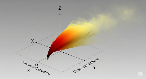
So, this Q and so we are integrating y from minus infinity to plus infinity, which mean this is the y-axis this is the x-axis is, this is the z-axis and this is the y-axis.
Detailed Explanation
We integrate concentration across all dimensions of the plume to ensure we account for how pollutants spread in space. By integrating over each spatial direction, we can quantify the total amount of pollutant present in the plume.
Examples & Analogies
Consider filling a balloon with air. You want to distribute air evenly throughout the balloon. Just like how you ensure every part has air, in this model, we ensure the pollutant concentration is spread across all dimensions.
Gaussian Distribution and Transformation of Variables
Chapter 6 of 8
🔒 Unlock Audio Chapter
Sign up and enroll to access the full audio experience
Chapter Content
Now, the Gaussian dispersion model looks quite similar to another equation known as a Gaussian distribution where the equation for normal distribution has a bell-shaped curve.
Detailed Explanation
The Gaussian dispersion model shares similarities with the Gaussian distribution, which is symmetrical and representative of how pollutant concentrations are expected to spread. By transforming variables to fit this form, we can analyze pollutant dispersion more effectively.
Examples & Analogies
Think of how light diffuses in water. Initially, light may be intense in one spot, but as it spreads out, the intensity diminishes, creating a bell-shaped silhouette. Similarly, concentrations of pollutants vary, being high at their source but tapering off symmetrically.
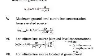
Identifying Maximum Concentration
Chapter 7 of 8
🔒 Unlock Audio Chapter
Sign up and enroll to access the full audio experience
Chapter Content
So, for which we look at an ideal plume. An ideal plume is nicely going in this kind of cone fashion. The cross-section looks like an ellipse or even a circle.
Detailed Explanation
An ideal plume's shape is essential in determining where maximum pollutant concentrations are likely to occur. The highest concentration typically aligns with the geometric center of the plume’s cross-section, which can be modeled mathematically for analysis.
Examples & Analogies
Imagine a flashlight beam creating a bright spot on the wall. The center of the beam has the most light; similarly, the center of a pollutant plume has the highest concentration, tapering off towards the edges.
Final Equation of Gaussian Dispersion Model
Chapter 8 of 8
🔒 Unlock Audio Chapter
Sign up and enroll to access the full audio experience
Chapter Content
So, this here is an important consideration that we are defining some parameters to fit this equation into a Gaussian format.
Detailed Explanation
The final equation for the Gaussian dispersion model incorporates different parameters that take into account the specific characteristics of the pollutant source and its environment, allowing for accurate predictions of concentration at various points in space.
Examples & Analogies
Think of a recipe that needs specific ingredients and measurements to taste good. Similarly, the Gaussian dispersion model needs various parameters to predict concentration accurately, ensuring the calculations reflect real-world outcomes.
Key Concepts
-
Steady-State Assumption: Concentration at a location remains constant over time.
-
Three-Dimensional Dispersion: Pollution spreads in x, y, and z directions.
-
Mass Conservation: Total mass released equals mass within the plume.
-
Gaussian Distribution: The concentration of pollutants follows a bell-curve shape.
-
Plume Behavior: Understanding plume variables is vital for pollution management.
Examples & Applications
An industrial plant emits pollutants at a stable rate every hour. The Gaussian model can predict downwind concentrations at various distances.
A study used the Gaussian dispersion model to assess the impact of traffic-related emissions in an urban area, illustrating peak concentrations at specific locations.
Memory Aids
Interactive tools to help you remember key concepts
Rhymes
In the plume where pollutants roam, Gaussian shapes help us find home.
Stories
Imagine a factory by a river; as pollutants rise, they form a plume, like a smoke signal finding its way.
Memory Tools
Remember 'CPT' - Constant Pollution Trickle for the steady-state assumption!
Acronyms
DAMP
Dispersion
Area
Mass
Predictions – key aspects of pollution modeling.
Flash Cards
Glossary
- Gaussian Dispersion Model
A mathematical model that predicts how pollutants disperse in the atmosphere based on Gaussian distribution.
- SteadyState Assumption
An assumption that concentration does not change with time at a fixed location.
- Mass Conservation
The principle that mass in a closed system must remain constant over time.
- Dispersion
The spreading of pollutants in the atmosphere due to various environmental factors.
- Plume
A visible or measurable trail of pollutants in the atmosphere, originating from a source.
Reference links
Supplementary resources to enhance your learning experience.