
Transformation of the Equation
Enroll to start learning
You’ve not yet enrolled in this course. Please enroll for free to listen to audio lessons, classroom podcasts and take practice test.
Interactive Audio Lesson
Listen to a student-teacher conversation explaining the topic in a relatable way.
Steady State Assumption
🔒 Unlock Audio Lesson
Sign up and enroll to listen to this audio lesson

Today, we will discuss the steady-state assumption in dispersion modeling. Can anyone tell me what steady-state means when we say the concentration does not change with time?

Does it mean that the concentration at a specific point remains constant?
Exactly! In the steady-state, the concentration at each point in space stays the same over time. This is essential for our Gaussian dispersion model.

But what if the emissions change? Would that affect the assumption?
Good question! If emissions or other parameters change over time, then we cannot use the steady-state assumption. Remember, average values help us deal with these fluctuations.
To remember this, think of the acronym SAFE - Steady At a Fixed Environment!

I like that! So it helps us simplify our calculations?
Exactly, it does! Now let's recap: in a steady state, concentrations remain constant over time and we use average values to manage fluctuations.
Integration and Dimensional Analysis
🔒 Unlock Audio Lesson
Sign up and enroll to listen to this audio lesson

Next, let’s look at how we integrate our dispersion model across different axes. Can anyone tell me the axes we usually consider?

I think we have the x, y, and z axes that represent different spatial directions.
Correct! So when we talk about integration, we derive limits that reflect our physical boundaries. For example, in the z-direction, we may integrate from 0 to infinity.
Why do we start at zero for z?
Because the plume cannot go below ground level, but can extend infinitely upwards. So, we incorporate this logic in our dimensional analysis.
Remember the mnemonic 'ZIG-ZAG' for limits: Zero In Ground, Zestful Above!
That’s helpful! How do we use these integrations in solving real problems?
The integrated equations will help us predict the pollutant concentrations effectively, depending on the mass flow and emitted rates.
Linking to Gaussian Distribution
🔒 Unlock Audio Lesson
Sign up and enroll to listen to this audio lesson
Now, let’s connect our derived equations to the Gaussian distribution model. Who can tell me why this connection is vital?
I believe the Gaussian distribution helps in visualizing how pollutants spread!
Exactly! The shape of the Gaussian curve shows how concentration diminishes with distance from the center of the plume.
What does the standard deviation signify here?
Great question! A higher standard deviation indicates a wider spread of pollutants, which correlates to lower peak concentrations. Remember, 'Width Wanes, Peak Pains!'—which means, as dispersion widens, the highest concentration diminishes.
So the Gaussian model aids in planning and estimating impacts?
Exactly! It is crucial for environmental assessment and regulatory compliance.
Boundary Conditions and Mass Conservation
🔒 Unlock Audio Lesson
Sign up and enroll to listen to this audio lesson
Finally, let’s discuss boundary conditions and mass conservation. Why do we need to ensure conservation of mass in our models?
Mass conservation would mean that we're accounting for all pollutants released into the environment!
Exactly! The total mass of pollutants must equal the rate of emission over time. We can use the general equation derived from our earlier discussions.
And how do we track the mass flow in our equations?
We relate the mass flow, Q, to the equations through integration across volume and ensuring total pollutant mass stays constant.
To remember this concept, think of ‘MASS MATTERS; it must never be scattered!’
That’s a catchy phrase! It reminds us that we need to track mass flow carefully.
Exactly! In summary, the boundary conditions help us formulate more accurate models ensuring mass conservation is always a priority.
Introduction & Overview
Read summaries of the section's main ideas at different levels of detail.
Quick Overview
Standard
The section elaborates on the transformation of the dispersion equation, focusing on the steady-state assumption that concentration does not change over time at a given location. It details how to integrate dispersion across three axes, the implications of utilizing average values, and how to derive a general solution incorporating boundary conditions and mass conservation principles.
Detailed
Transformation of the Equation
In this section, we explore the transformation of the dispersion equation, fundamental to understanding pollutant concentration in fluid dynamics. The dialogue initiates with assumptions regarding steady-state conditions, notably that the concentration remains constant over time at spatial points, shaped by consistent emission rates and physical properties. This assumption is paramount for employing the Gaussian dispersion model, where variations over time necessitate different modeling approaches.
Key Concepts Explained:
- Steady State Assumption: Concentration at any location does not change with time, leading to simplifications in analytic modeling
- General Solution: We derive a general solution through multiple constants across three dimensions, encapsulating all boundary conditions and leveraging mass conservation principles.
- Gaussian Distribution: The section frames the pollutant dispersal model akin to Gaussian distribution, indicating how concentration relates to spatial distribution.
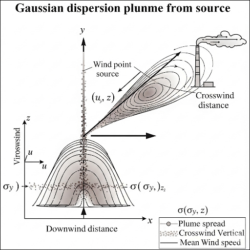
By utilizing dimensional analysis, particularly integrating over specific axes with varying limits, we can delineate the characteristics of a pollutant plume, encompassing its expansion in three-dimensional space as it disperses. This lays groundwork for understanding how concentration varies both spatially and in terms of emission dynamics in atmospheric environments.
Youtube Videos


Audio Book
Dive deep into the subject with an immersive audiobook experience.
Steady State Assumption
Chapter 1 of 4
🔒 Unlock Audio Chapter
Sign up and enroll to access the full audio experience
Chapter Content
Now here we make two assumptions, one is a steady state assumption you don’t have to do this but for that Gaussian dispersion model that we generally present we use the steady state assumptions where we say &)!" = 0, which means that at any point in time the concentration is &* thesame, atanylocationyoumeasureitconcentrationwillnotchangewithtime.
Detailed Explanation
In this part, the content discusses an important assumption we make when modeling dispersion, known as the steady state assumption. This means that when we observe a specific location over time, the concentration of a substance (like a pollutant) remains constant. It can vary from one location to another, but it does not change over time at a specific point. This assumption is crucial for simplifying the mathematical models we use to predict how substances disperse in the environment.
Examples & Analogies
Think of it like a slowly leaking faucet. If you measure the water level in a container under the faucet, while the water is slowly dripping at a constant rate, you'd find that the level stays consistent over time until you turn off the faucet or change the drip rate. Similarly, in a steady state assumption, we assume that the rate of pollutant release and the environmental conditions that influence this concentration remain steady.
Neglecting Bulk Flow
Chapter 2 of 4
🔒 Unlock Audio Chapter
Sign up and enroll to access the full audio experience
Chapter Content
Thesecondthingthatwedoissincewealreadyhaveuxbulkflowinginthexdirection.Weneglectthisdxterm,sothisentirethingreducestothissimplerequationthisiswherewestoppedlastclass.
Detailed Explanation
Here, the text mentions neglecting certain terms associated with bulk flow in the x-direction (the direction in which the substance is primarily moving). This simplification allows us to reduce complex equations into simpler forms that are easier to work with, making it more feasible to find solutions to our models. By eliminating minor effects, we can focus on the primary behavior of the pollutant dispersion.
Examples & Analogies
Imagine you're trying to calculate the flow of a river. If you were to include every little rock and pebble in the waterway's path, your calculations would become incredibly complex. Instead, you can just focus on the river's main flow, allowing you to predict its behavior with much less complication.
General Solution and Mass Conservation
Chapter 3 of 4
🔒 Unlock Audio Chapter
Sign up and enroll to access the full audio experience
Chapter Content
Now, the general solution for this, this is an equation there are solutions are already there. This form, you do separation of variables and do all that. You will get an equation of this form...
Detailed Explanation
The content goes on to discuss finding a general solution to the equation describing the dispersion of pollutants. It involves using the principle of mass conservation, which states that the mass of pollutants must equal the total mass emitted over a specified volume. When applying these principles, we can derive equations that describe the spread of contaminants in the air and allow us to make predictions based on known quantities.
Examples & Analogies
Think about how water flows through different shapes of containers. No matter the shape, the amount of water pouring in will eventually fill the space available, demonstrating mass conservation. Similarly, understanding how the concentration of pollutants behaves in the atmosphere relies on the concept that whatever is released must conform to the surrounding volume.
The Gaussian Distribution
Chapter 4 of 4
🔒 Unlock Audio Chapter
Sign up and enroll to access the full audio experience
Chapter Content
Now, the Gaussian dispersion model in its preliminary form looks like this; this equation here doesn’t look it looks almost the same but is not in the same format.
Detailed Explanation
Here, the text discusses how the Gaussian dispersion model aligns with a standard Gaussian (bell curve) format, but requires transformation to fit the model accurately. It elaborates on how this mathematical form helps to describe the spread and concentration of the pollutant in three-dimensional space, factoring in various dispersion directions.
Examples & Analogies
Imagine a loud sound from a speaker. Right next to the speaker, the sound is loudest, and as you move away, the sound gradually becomes softer. The 'spread' of sound can resemble a Gaussian distribution: more intense concentration (loudness) in the center and tapering off on the edges. In a similar way, pollutants disperse most densely at the source before gradually becoming less concentrated further away.
Key Concepts
-
Steady State Assumption: Concentration at any location does not change with time, leading to simplifications in analytic modeling
-
General Solution: We derive a general solution through multiple constants across three dimensions, encapsulating all boundary conditions and leveraging mass conservation principles.
-
Gaussian Distribution: The section frames the pollutant dispersal model akin to Gaussian distribution, indicating how concentration relates to spatial distribution.
-
-
By utilizing dimensional analysis, particularly integrating over specific axes with varying limits, we can delineate the characteristics of a pollutant plume, encompassing its expansion in three-dimensional space as it disperses. This lays groundwork for understanding how concentration varies both spatially and in terms of emission dynamics in atmospheric environments.
Examples & Applications
An example of a steady-state assumption in air pollution modeling, where pollutant levels are assessed over a consistent time period.
A Gaussian distribution example can be seen in the spread of pollen in the air, illustrating high concentrations close to the source and tapering off further away.
Memory Aids
Interactive tools to help you remember key concepts
Rhymes
In steady state, pollutants wait, concentration won’t hesitate, at each place, maintain the pace!
Stories
Imagine a factory releasing smoke; for every puff, the sky remains the same shade. This is like a firm steady state where we keep track of the smoke's spread over time.
Memory Tools
Remember 'MASS MATTERS' to focus on conservation of mass in pollution equations.
Acronyms
Use SAFE to recall Stays At a Fixed Environment for steady state!
Flash Cards
Glossary
- Steady State Assumption
The assumption that the concentration of a pollutant does not change over time at a specified location.
- Gaussian Distribution
A statistical distribution where the concentration profile resembles a bell curve, illustrating the spread of pollutants.
- Integration
The mathematical process of summing terms over a continuous range to analyze total dispersion within specified limits.
- Boundary Conditions
Constraints that define the limits or edges of a system being modeled, crucial for solving mathematical equations.
- Mass Conservation
A principle stating that the total mass must remain constant throughout a system unless acted on by an external force.
Reference links
Supplementary resources to enhance your learning experience.