
Determining the Center of the Plume
Enroll to start learning
You’ve not yet enrolled in this course. Please enroll for free to listen to audio lessons, classroom podcasts and take practice test.
Interactive Audio Lesson
Listen to a student-teacher conversation explaining the topic in a relatable way.
Understanding Steady-State Assumptions
🔒 Unlock Audio Lesson
Sign up and enroll to listen to this audio lesson

Today, we are going to discuss the steady-state assumption in Gaussian dispersion models. Can anyone tell me why this assumption is crucial?

I think it’s because it simplifies the calculations and helps us assume that the concentration doesn’t change over time at a location.
Correct! By assuming steady-state, we expect the system parameters, like emission rates, to remain constant. What happens if these parameters change over time?

Then we can’t use the steady-state model anymore, right?
Exactly! So we need to be cautious using this model. Remember—steady state means no temporal changes in concentration.

Can you give us a mnemonic for remembering steady state?
Sure! Think of 'Steady State' like 'Steady as She Goes.' This means everything is constant and calm, no ups and downs in concentration over time.
To summarize, in a steady state, nothing changes in time at any location—this includes emission rates and pollutant properties.
Mass Conservation in Plume Behavior
🔒 Unlock Audio Lesson
Sign up and enroll to listen to this audio lesson

Next, let's discuss mass conservation. Why is this concept vital when working with plume dispersion models?

Because we need to ensure that the total mass of pollutants released matches the mass present in the plume!
Exactly! The equation we need shows Q, the pollutant release rate, equals the mass flow per volume. Can anyone recall how we express this mathematically?
It involves integrating over the volume of the plume, right?
Correct! We integrate from negative to positive infinity in the y-axis, but in the z-direction, it’s constrained by the ground at z = 0. This allows us to encapsulate the full volume of the plume.
So, how do we calculate this for a specific situation?
That’s where understanding boundary conditions comes into play. They give us limits and conditions for our integrations. Remember, the plume behavior must adhere to conservation laws.
In summary, mass conservation ensures that all emissions are accounted for in our models, fulfilling key relationships in the plume’s behavior.
Gaussian Distribution and Plume Center Identification
🔒 Unlock Audio Lesson
Sign up and enroll to listen to this audio lesson
Now, let’s relate Gaussian distribution to our plume model! How does this connect with our discussions on concentration profiles?
I guess the Gaussian distribution tells us how pollutants spread out in a plume?
Exactly! The equation for the Gaussian distribution is structured similarly to the environment’s concentration distribution. What defines the concentration's peak?
It's at the center of the plume, right? Where the concentration is highest?
Correct! This point is crucial as it helps us define the coordinates for the highest concentration. Let’s work through an equation to illustrate this. What transformations do we need?
Do we need to account for the spread in both the y and z directions?
Yes! This gives us sigma values for y and z necessary for our calculations. Great connection there!
To summarize, recognizing that the Gaussian distribution helps define where the plume concentration peaks is foundational in our modeling.
Introduction & Overview
Read summaries of the section's main ideas at different levels of detail.
Quick Overview
Standard
The section details how to approach the dispersion of pollutants in three dimensions, making steady state assumptions. It discusses how to derive concentrations relying on basic principles of mass conservation and the Gaussian distribution, ultimately leading to identifying the center of a plume.
Detailed
In this section, we delve into determining the concentration profiles within a pollutant plume using the Gaussian dispersion model. We begin with the assertion that under steady-state conditions, concentration remains constant over time at any given location. This assumption requires the emission rates and plume characteristics to remain unchanged, allowing for an analysis that simplifies calculations. We then explore the dispersion across the three dimensions of the plume, enabling a straightforward integration approach across defined limits. By applying mass conservation and the Gaussian distribution, we define the highest concentration's location (the plume's center) based on flow rate and dispersion coefficients. The simplification into a single equation captures boundary conditions and leads to a general solution related to the plume's behavior depending on its source characteristics.
Youtube Videos

![[ADI] PLUME BEHAVIOUR (ENVIRONMENT ENGINEERING) EXPLAINED (CE)!!! In Hindi](https://img.youtube.com/vi/pUaqNCqAgFc/mqdefault.jpg)


Audio Book
Dive deep into the subject with an immersive audiobook experience.
Steady State Assumptions
Chapter 1 of 4
🔒 Unlock Audio Chapter
Sign up and enroll to access the full audio experience
Chapter Content
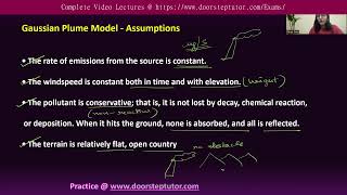
We make two assumptions, one is a steady state assumption you don’t have to do this but for that Gaussian dispersion model that we generally present we use the steady state assumptions where we say &)! = 0, which means that at any point in time the concentration is &* the same, at any location you measure it concentration will not change with time. It will be different with space but it will not change with time.
Detailed Explanation
The first assumption relates to what is called a steady state. When we talk about a steady state, we mean that the concentration of pollutants does not change over time at specific locations. This means if we measure a location today, its pollutant concentration will remain the same at that point tomorrow and the next day, provided that other conditions like emissions and surrounding environmental factors remain constant. However, the concentration can vary across different locations in the plume.
Examples & Analogies
Imagine a river where the water quality (pollutants) is measured at a specific point. If we say it's in a steady state, we expect the measurements to be the same every day at that exact location, unless something changes upstream. However, the quality might differ just a few meters downstream due to different inputs.
Constants and Boundary Conditions
Chapter 2 of 4
🔒 Unlock Audio Chapter
Sign up and enroll to access the full audio experience
Chapter Content
So, we are saying Q is the rate of pollutant release equals u multiplied by dy and dx, ux into dy into dz will be if you look at the dimensions L by T into L into L into M by L cubed this is M by L cubed equals M by T.
Detailed Explanation
In this part, we discuss the relationship between the rate of pollutant release (Q) and the flow rates in three dimensions (x, y, z). By integrating the factors, we assess how the volume of polluted air or water is quantified considering the pollutant's movement and dispersion in the environment. This involves concrete mathematical relations showing that the total mass present is derived from the pollution rate divided by how it disperses in space.
Examples & Analogies
Think of it as trying to calculate how far the scent of a cake will spread in a room after you take it out of the oven. The rate at which the cake scent spreads (Q) can be pictured as the constant rate of release, while its movement in the room (dy, dx, dz) determines how broadly the scent covers the area.
Gaussian Dispersion Model
Chapter 3 of 4
🔒 Unlock Audio Chapter
Sign up and enroll to access the full audio experience
Chapter Content
But there is something that people have gone ahead and manipulated this particular equation with the ideal assumption that if you look at this equation, this is very similar to another equation which is called as a Gaussian distribution or a normal distribution.
Detailed Explanation
Here, we introduce the Gaussian dispersion model, which suggests that the distribution of the pollutant concentrations can be visually represented as a bell-shaped curve, known as a Gaussian distribution. This implies that, in a perfectly ideal scenario, the highest concentration of pollutants is found at the center of the plume, tapering off symmetrically on either side.
Examples & Analogies
Imagine throwing a pebble into a still pond; the ripples spread out in concentric circles. In this case, the point where the pebble landed is akin to the highest concentration point in a Gaussian model—where the disturbances (pollutants) are greatest. As you move away from this point, the impact (or concentration) lessens, similar to how the ripples dissipate.
Center of the Plume
Chapter 4 of 4
🔒 Unlock Audio Chapter
Sign up and enroll to access the full audio experience
Chapter Content
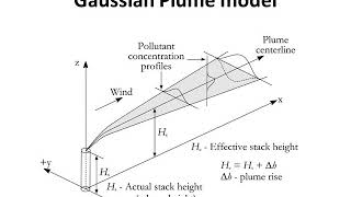
So, the highest concentration occurs at some value of z or y, where z represents the height and y represents the lateral spread.
Detailed Explanation
This section underscores the significance of finding the center of the plume, where the pollutant concentration is at its maximum. Depending on the orientation of the pollution source, the highest concentration could be at different vertical (z) or horizontal (y) positions, emphasizing that pollutants don't just spread uniformly—they follow specific dispersion patterns.
Examples & Analogies
Think about standing in front of a campfire. The smoke is thickest directly above the fire, where the heat rises. The higher you go (z-axis), the thinner the smoke becomes. Similarly, if you were to measure the smoke's presence laterally (y-axis) close to the fire, you'd notice more concentration near the flames than further away.
Key Concepts
-
Steady State: Concentration remains constant over time at a fixed location.
-
Mass Conservation: Mass in a closed system is conserved.
-
Gaussian Distribution: Illustrates how pollutants spread out like a bell curve.
-
Boundary Conditions: Essential for defining limits of mathematical models.
-
Concentration Peak: The location within the plume with the highest pollutant concentration.
Examples & Applications
An ideal plume expands symmetrically in all directions from its source, with the highest concentration located directly above the source.
In real-world applications, wind speed affects plume dispersion, altering the shape and dimensions of the Gaussian distribution curve applied.
Memory Aids
Interactive tools to help you remember key concepts
Rhymes
In a steady state, the flow won’t sway, Concentrations remain, come what may!
Stories
Imagine a steady stream of water flowing uniformly down a hill without any rocks to disturb its path - that’s like a Gaussian plume in a steady state.
Memory Tools
C-C-M-B for remembering Concentration-Center-Mass-Boundaries in modeling.
Acronyms
G.D.P. – Gaussian Distribution Peaks, to highlight where concentrations are highest.
Flash Cards
Glossary
- Gaussian dispersion
A model that describes how pollutants disperse in the atmosphere, characterized by a bell-shaped curve.
- Steady state
Condition where concentration does not change with time at a particular location.
- Mass conservation
A principle that states that mass is neither created nor destroyed in a closed system.
- Boundary conditions
Conditions that must be satisfied at the edges of the domain in a mathematical model.
- Concentration peak
The point in a pollutant dispersion where the concentration of the pollutant is highest.
- Dimensions of dispersion
The directions (x, y, and z) in which the pollutant plume expands.
Reference links
Supplementary resources to enhance your learning experience.