
Example Problem 4
Enroll to start learning
You’ve not yet enrolled in this course. Please enroll for free to listen to audio lessons, classroom podcasts and take practice test.
Interactive Audio Lesson
Listen to a student-teacher conversation explaining the topic in a relatable way.
Bernoulli's Equations Application
🔒 Unlock Audio Lesson
Sign up and enroll to listen to this audio lesson

Today, we will discuss how Bernoulli's equations can be applied in fluid dynamics to analyze various flow problems. Can anyone remind me what Bernoulli's principle states?

It states that an increase in the speed of the fluid occurs simultaneously with a decrease in pressure or potential energy.
Exactly! So, when we apply Bernoulli’s equation between points in a flow, we are looking at the conservation of energy principle for fluids.

How do we know which points to choose for calculation?
Great question! We typically choose points where we can measure velocities and pressures. For example, in a horizontal jet striking a plate, those points might be where the flow enters and exits the system.

And when we use these equations, we can derive the force on the plate?
Exactly! By calculating the momentum flux, we can quantify the force the fluid exerts on the plate.
Remember, from Bernoulli’s perspective, we’re looking at pressure force, inertia, and friction in a balanced way.
Reynolds Transport Theorem
🔒 Unlock Audio Lesson
Sign up and enroll to listen to this audio lesson

Let's talk about the Reynolds transport theorem. Does anyone know how it simplifies our momentum calculations?
Isn't it used to convert the integral form of the conservation laws into a differential form?
Good! It allows us to relate the rate of change of momentum within a control volume to the momentum flux across its boundaries. This is crucial for analyzing jet flows.
So we can express the forces in terms of inflow and outflow?
Exactly! We need to equate the influx and outflux components to evaluate the net force. Can you see how this relates to our earlier discussions on velocity and area?
Yes, it helps us understand how to calculate the effective areas in our applied formulas.
Exactly! By carefully selecting our control volume, we can derive insightful momentum relationships.
Horizontal Jet Analysis
🔒 Unlock Audio Lesson
Sign up and enroll to listen to this audio lesson
Let’s apply these concepts to a horizontal jet striking a plate—what should we start with?
We should identify the flow rate and velocity at the entry and exit points, right?
Exactly! Knowing the flow rate allows us to compute the resulting velocities which we can plug back into Bernoulli’s equation.
And then calculate momentum and force?
Yes! We'll calculate momentum in both directions—x and y—to determine the total force exerted on the plate. Remember, we use the equation of continuity for that as well!

What if we consider an angle, like in our next example?
When the jet impacts at an angle, we must resolve the components to account for horizontal and vertical forces separately, still using the same principles.
Venturimeter Applications
🔒 Unlock Audio Lesson
Sign up and enroll to listen to this audio lesson
Now let's explore the venturimeter example. Does anyone know why we use it for measuring flow rates?
It helps determine how the velocity changes with pressure differences.
Correct! By applying Bernoulli’s equation to a venturimeter setup, we can find the discharge coefficient using measured pressure differences.
How do we relate the areas and velocities in a venturimeter?
We employ the principle of continuity! The equation A1V1 = A2V2 helps us connect the geometries at the two points.
And the discharge coefficient comes from comparing actual and theoretical flow rates?
Exactly! That’s how we validate our measurements against theoretical expectations.
Introduction & Overview
Read summaries of the section's main ideas at different levels of detail.
Quick Overview
Standard
In this section, we explore how to apply Bernoulli’s equations and linear momentum equations to analyze fluid flow problems, specifically focusing on calculating force components and resultant forces through worked examples such as a horizontal jet striking a vertical plate and a venturimeter.
Detailed
In this chapter, we delve into the practical applications of Bernoulli's equations in fluid dynamics, particularly as it pertains to computing flow rates and resulting forces in various scenarios. We start with a problem involving a horizontal flow jet impacting a vertical plate, demonstrating the application of Reynolds transport theorems to simplify linear momentum equations. The formulation allows us to express the balance of forces through the control volume encompassing the jet and plate. Further, we analyze momentum flux in both x and y directions to derive resultant forces. The section culminates with a venturimeter example, showcasing how to compute pressure differences and discharge coefficients through Bernoulli’s principle. By methodically applying theoretical equations, we gain insights into real-world flow dynamics.
Youtube Videos


Audio Book
Dive deep into the subject with an immersive audiobook experience.
Understanding the Flow Conditions
Chapter 1 of 5
🔒 Unlock Audio Chapter
Sign up and enroll to access the full audio experience
Chapter Content
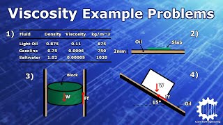
In this case, there is a horizontal jet of the flow with angle theta striking a vertical plate, and the flow distribution here is Q naught, with the flow at this point equal to 0.25 times the Q naught value. We try to find out what could be the theta value when the impact loss is neglected.
Detailed Explanation
This excerpt sets the stage for the problem. We have a horizontal jet of fluid that impacts a vertical plate at an angle theta. To analyze this situation, we denote the flow rate as Q naught. At one point of interest, the flow is reduced to 25% of Q naught. The goal here is to determine the angle theta under the assumption that impact losses are negligible, simplifying our calculations.
Examples & Analogies
Think of this like water from a garden hose spraying against a wall. If you tilt the hose (angle theta), the water hits the wall differently. In this scenario, we're trying to figure out the best angle to spray the water such that most of it splashes back rather than drips down.
Flow Classifications
Chapter 2 of 5
🔒 Unlock Audio Chapter
Sign up and enroll to access the full audio experience
Chapter Content
The flow can be classified as steady, incompressible, one-dimensional, and frictionless, meaning we neglect any frictional component due to the vertical plate. Given these conditions, we will apply Bernoulli’s equations for this case.
Detailed Explanation
The passage describes key characteristics of the fluid flow around the plate. Steady flow means that the fluid properties do not change over time. Incompressible flow indicates that the density of the fluid remains constant (which is typically valid for liquid flows). One-dimensional flow simplifies our calculations to one direction, even if it visually appears two-dimensional. Frictionless flow assumes that there are no losses due to friction with the plate, further simplifying our analysis as we apply Bernoulli’s equations.
Examples & Analogies
Imagine a smooth slide at a water park. The water flows steadily down the slide (steady flow). The slide is made to minimize any bumps that could slow down the water (frictionless). And even though the slide bends and twists, we can view the water flow as if it’s just moving straight down (one-dimensional).
Applying Bernoulli’s Equations
Chapter 3 of 5
🔒 Unlock Audio Chapter
Sign up and enroll to access the full audio experience
Chapter Content
To apply Bernoulli’s equations, we can draw streamlines between points in the flow. At point 1, the pressure is equal to atmospheric pressure, and at point 2, we consider the velocities and heights to establish equations relating them.
Detailed Explanation
In applying Bernoulli's principle, we analyze the energy balance along the streamline from one point to another. Since point 1 is at atmospheric pressure, we can equate the potential energy and kinetic energy changes between the two points using Bernoulli’s equation. For this case, because there are no friction losses, Bernoulli’s equation helps us relate the pressure and velocity at different points along the fluid's path.
Examples & Analogies
Think of the difference in water pressure when using a sprinkler system. As water travels through the pipes, it moves from a high-pressure area to a lower-pressure area, changing its speed. Bernoulli’s equation essentially captures that relationship between pressure and velocity as the water flows through.
Calculating the Angle Theta
Chapter 4 of 5
🔒 Unlock Audio Chapter
Sign up and enroll to access the full audio experience
Chapter Content
Next, we use linear momentum equations to compute the theta value, noting that the sum of the forces acting on the object should equal zero, as it is stationary.
Detailed Explanation
Here, we are integrating the principles of momentum and equilibrium. We establish that the forces acting on the control volume are balanced, allowing us to set up the equations that describe how the fluid's momentum affects the angle theta. By substituting the flow conditions into the linear momentum equations, we solve for theta, providing insight into how the flow direction influences the impact on the plate.
Examples & Analogies
When throwing a ball, you need to choose the right angle to make it reach your friend across the field. If you throw too high or low, the ball either travels too far or lands short. Similarly, in our fluid flow, determining the perfect angle (theta) to maintain balance is crucial for optimal flow performance.
Final Equation for Theta
Chapter 5 of 5
🔒 Unlock Audio Chapter
Sign up and enroll to access the full audio experience
Chapter Content
By substituting known values into our equations, we find the sine of theta corresponds to 0.5, which indicates that theta is equal to 30 degrees, which is the solution to our problem.
Detailed Explanation
After deriving and simplifying our equations through the linear momentum approach, we ultimately calculate that sin(theta) equals 0.5. Since the sine of 30 degrees is 0.5, we conclude that the specific angle theta which results in a stationary system is 30 degrees. It encapsulates our findings and provides a clear measure of how the jet impacts the plate.
Examples & Analogies
Just like when you’re aiming to hit a target with a slingshot, the angle you hold it makes a big difference in where the shot lands. Here, we calculated the angle of impact that balances our fluid system, ensuring the water flows as intended without unnecessary splatter.
Key Concepts
-
Flow Rate: The volume of fluid passing through a surface per unit time.
-
Momentum: A property of moving mass that affects collisions and changes in velocity.
-
Bernoulli's Principle Application: The use of Bernoulli’s equation to analyze pressure and velocity relations in fluid flow.
-
Control Volume Analysis: Applying momentum equations within a defined space to assess forces and flux.
Examples & Applications
Example of fluid flowing from a larger diameter pipe to a smaller one, illustrating increased velocity and decreased pressure.
Demonstration of calculating forces exerted by a fluid jet on an impact surface, using Bernoulli's equation.
Memory Aids
Interactive tools to help you remember key concepts
Rhymes
When flow is quick, pressure might drop, Bernoulli's principle helps us nab the spot.
Acronyms
B.E. – Bernoulli’s Energy; relates speed and pressure to enlighten you all.
Stories
Imagine a runner speeding down a track. As they run faster, the pressure from the air decreases, just like in a fluid stream; it’s a real-life application of Bernoulli’s principles in motion.
Memory Tools
Remember: 'Low V means High P' — Low velocity corresponds to high pressure in fluid dynamics terms!
Flash Cards
Glossary
- Bernoulli's Equation
A principle that describes the conservation of energy in fluid dynamics, linking speed, pressure, and height.
- Linear Momentum
The product of an object's mass and its velocity, representing the quantity of motion an object possesses.
- Reynolds Transport Theorem
A theorem that provides a relationship between the time rate of change of some quantity within a control volume and the flux of that quantity across the control surface.
- Discharge Coefficient
A dimensionless number used to characterize the discharge potential of a flow meter or nozzle.
- Momentum Flux
The rate of transfer of momentum through a surface per unit area.
- Control Volume
A defined volume in space through which fluid can flow, used for analysis in fluid dynamics.
Reference links
Supplementary resources to enhance your learning experience.