
Rectangular Membrane, Use of Double Fourier Series
Enroll to start learning
You’ve not yet enrolled in this course. Please enroll for free to listen to audio lessons, classroom podcasts and take practice test.
Interactive Audio Lesson
Listen to a student-teacher conversation explaining the topic in a relatable way.
Understanding the Two-Dimensional Wave Equation
🔒 Unlock Audio Lesson
Sign up and enroll to listen to this audio lesson

The two-dimensional wave equation describes how vibrations in a rectangular membrane move over time. Can anyone tell me what \( u(x,y,t) \) represents in this equation?

Is it the displacement at point (x,y) and time t?
Exactly! Now, what do you think the parameters \( c \) stands for?

It’s the wave speed, right?
Correct! This speed relates to the tension and mass density of the membrane. Now, why are the boundary conditions important?

They help define how the membrane is fixed at the edges.
Exactly! They set the limits for our solutions. Remember those conditions: \( u(0,y,t) = 0 \) and so forth. Great job!
Separation of Variables
🔒 Unlock Audio Lesson
Sign up and enroll to listen to this audio lesson

Now we assume a solution of the form \( u(x,y,t) = X(x)Y(y)T(t) \). Can anyone explain why we separate the variables?

To make the differential equation easier to solve by breaking it into manageable parts?
That's right! This allows us to consider each component individually. When we substitute, we set each side equal to a constant, right?
Yes, we can set it to \(-\lambda\).
Good memory! Each spatial part correlates to an equation that helps find eigenvalues and eigenfunctions. Who can define what eigenvalues are in this context?
They are the values that determine the modes of vibration of the membrane.
Exactly! As we identify those modes, we begin to see the actual shapes that the membrane can take during vibration.
Full Solution and Application
🔒 Unlock Audio Lesson
Sign up and enroll to listen to this audio lesson
We can combine our solutions to get the full representation of the membrane's vibration, which ends up looking like a double Fourier series. Why do you think practical engineers care about these solutions?
They need to ensure structures can handle vibrations from loads, right?
Absolutely! Vibration analysis is crucial for safety and stability in civil engineering. Can anyone name a structure that might use these principles?
Bridges, especially during earthquakes!
Spot on! Understanding these vibrations helps engineers design better structures. Let's wrap it up— who can summarize the main solution approach we've learned?
We separate variables, solve for eigenfunctions, and combine those to analyze the membrane’s vibration modes.
Perfect summary! Keep these principles in mind as we proceed.
Introduction & Overview
Read summaries of the section's main ideas at different levels of detail.
Quick Overview
Standard
In this section, we explore the dynamics of a rectangular membrane governed by the two-dimensional wave equation, focusing on the solution techniques involving separation of variables and double Fourier series. Key findings include the determination of different modes of vibration and their applications in civil engineering.
Detailed
Detailed Summary
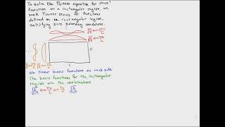
This section discusses the vibration of rectangular membranes, essential in structural and civil engineering. A rectangular membrane, typically seen in applications like vibrating plates, is modeled using the two-dimensional wave equation represented as:
$$
\frac{\partial^2 u}{\partial t^2} = c^2 \left( \frac{\partial^2 u}{\partial x^2} + \frac{\partial^2 u}{\partial y^2} \right)
$$
where \( u(x,y,t) \) is the displacement, and \( c \) is the wave speed dependent upon the membrane's tension and mass density. Given the fixed boundaries of the membrane (e.g., \( u(0,y,t) = u(a,y,t) = u(x,0,t) = u(x,b,t) = 0 \)), we also outline the initial conditions necessary for the solution.
The solution strategy involves using the method of separation of variables, postulating a solution of the form: \( u(x,y,t) = X(x)Y(y)T(t) \). This leads us to establish three distinct equations for spatial and temporal components from which we can derive solutions involving sinusoidal functions. Each mode of vibration has a corresponding eigenvalue that reflects its complexity and behavior under dynamic loads.
The final comprehensive solution employs double Fourier series, combining the solutions of both spatial and temporal components. The section emphasizes the significance of this method in analyzing various real-world structures, such as bridge decks and seismic responses, allowing for precise understanding and application in engineering design.
Youtube Videos
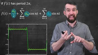
![Application of Fourier Series [ Square or rectangular wave ] .](https://img.youtube.com/vi/qx3bS1XhLaw/mqdefault.jpg)

Audio Book
Dive deep into the subject with an immersive audiobook experience.
Introduction to Rectangular Membranes
Chapter 1 of 15
🔒 Unlock Audio Chapter
Sign up and enroll to access the full audio experience
Chapter Content
In structural and civil engineering, understanding how membranes (like vibrating plates, stretched rectangular sheets, etc.) behave under various conditions is crucial for design and analysis. A rectangular membrane is a two-dimensional object that can oscillate or vibrate when disturbed. Mathematically, its motion is governed by the two-dimensional wave equation, and one of the most powerful methods for solving such partial differential equations over rectangular domains is the double Fourier series.
Detailed Explanation
This chunk introduces the concept of rectangular membranes as essential components in engineering. These membranes are two-dimensional surfaces that can vibrate, similar to a drum skin when struck. Their vibration patterns are described mathematically using the two-dimensional wave equation, a fundamental equation in physics that describes how waves propagate through a medium. The double Fourier series is a mathematical method used to find solutions to this equation for membranes with specific shapes (rectangular in this case).
Examples & Analogies
Think of a trampoline as a simple analogy. When you jump on a trampoline, it vibrates, and the patterns of those vibrations can be predicted mathematically, much like the vibrations of rectangular membranes. Engineers need to understand how these surfaces will behave to design safe and effective structures, similar to how a trampoline needs to be built to support weight without breaking.
The Two-Dimensional Wave Equation
Chapter 2 of 15
🔒 Unlock Audio Chapter
Sign up and enroll to access the full audio experience
Chapter Content
The transverse vibration u(x,y,t) of a rectangular membrane stretched tightly and fixed at the boundary is governed by the two-dimensional wave equation: ∂²u / ∂t² = c² (∂²u / ∂x² + ∂²u / ∂y²), where: • u(x,y,t): displacement of the membrane at point (x,y) and time t, • c: wave speed, depending on the tension and mass density of the membrane. The rectangular membrane has dimensions 0 < x < a, 0 < y < b, and its edges are held fixed, leading to boundary conditions: u(0,y,t)=u(a,y,t)=u(x,0,t)=u(x,b,t)=0. Additionally, the initial conditions are: u(x,y,0)=f(x,y), ∂u/∂t|t=0=g(x,y), where f(x,y) is the initial shape and g(x,y) is the initial velocity distribution.
Detailed Explanation
This chunk introduces the two-dimensional wave equation that describes how the membrane vibrates. The equation links the second derivatives of displacement with respect to time and space, reflecting how changes in time affect the position of the membrane, considering the tension and density. This leads to specific boundary conditions where the edges of the membrane (at x=0, x=a, y=0, and y=b) must remain fixed (i.e., the displacement is zero at these edges). Additionally, initial conditions detail how the membrane starts vibrating from an initial shape (f(x,y)) and an initial velocity distribution (g(x,y)).
Examples & Analogies
Consider the surface of a calm pond as an analogy. When a stone is thrown into the water, it creates ripples (vibrations) that spread out from the point of impact. The behavior of these ripples can be modeled similarly to the vibrations of a membrane using equations. Just like the water's surface returns to a flat state when the ripples fade away, the membrane returns to its boundary conditions after vibrations cease.
Solution by Separation of Variables
Chapter 3 of 15
🔒 Unlock Audio Chapter
Sign up and enroll to access the full audio experience
Chapter Content
We assume a solution of the form: u(x,y,t)=X(x)Y(y)T(t). Substituting into the wave equation: ... Since the left side depends only on t and the right side only on x and y, both must equal a constant, say −λ. We then separate again for spatial parts: ... Further separation gives: 1/X d²X/dx² + 1/Y d²Y/dy² + 1/c²T d²T/dt² = -λ. Then the time equation becomes: d²T/dt² + c²(α² + β²)T = 0.
Detailed Explanation
In this chunk, we discuss the technique of 'separation of variables,' where we look for solutions of the form that separates variables into distinct functions pertaining to x, y, and t. By substituting this assumed solution into the wave equation, we can derive separate equations for each variable. Eventually, this leads to an independent time equation that describes how time impacts the displacement of the membrane. The separation constant λ helps us connect all the equations together.
Examples & Analogies
Imagine trying to solve a jigsaw puzzle. Each piece must fit together to form the complete picture. Similarly, in the separation of variables, we're breaking down a complex problem (the wave equation) into smaller, manageable pieces. Each piece (X(x), Y(y), T(t)) can be solved individually and then combined to see the bigger picture (the overall vibration of the membrane).
Solving the Spatial Equations
Chapter 4 of 15
🔒 Unlock Audio Chapter
Sign up and enroll to access the full audio experience
Chapter Content
(i) Solving for X(x): d²X/dx² + α²X = 0 with boundary conditions: X(0)=X(a)=0 Solution: X(x)=sin(nπx/a), α = nπ/a, n=1,2,3,... (ii) Solving for Y(y): d²Y/dy² + β²Y = 0 with boundary conditions: Y(0)=Y(b)=0 Solution: Y(y)=sin(mπy/b), β = mπ/b, m=1,2,3,...
Detailed Explanation
In this chunk, we delve into how to solve the equations for the spatial dimensions (X and Y) of the membrane. We apply the standard boundary conditions that specify how these functions must behave at the edges. For X(x), we derive a solution involving sine functions, which are fundamental in wave mechanics due to their oscillatory nature. The same process applies to Y(y), resulting in another sine solution. These sine functions are critical as they represent possible modes of vibration along each axis.
Examples & Analogies
Consider the strings of a guitar. When you pluck a string, it vibrates in specific patterns that correspond to its length, tension, and mass. The solutions we find for X(x) and Y(y) are similar to the vibrations of guitar strings. Different combinations of these vibrations create various musical notes, much like how we create various vibration modes in a membrane through our solutions.
Solving the Time Equation
Chapter 5 of 15
🔒 Unlock Audio Chapter
Sign up and enroll to access the full audio experience
Chapter Content
d²T/dt² + c²(α² + β²)T = 0. Let: ω = c√(α² + β²). Then: T(t)=A cos(ωt)+B sin(ωt).
Detailed Explanation
In this section, we solve the time-dependent part of the equation. The resulting second-order differential equation describes oscillatory motion, where the solutions involve cosine and sine functions. The terms A and B represent amplitudes for the respective cosine and sine components, which capture how the system vibrates over time. The variable ω, known as the angular frequency, indicates how fast these oscillations occur, determined by the speed of the wave and the parameters from the spatial equations.
Examples & Analogies
Think about a swing at a playground. When you push a swing, it moves back and forth in a specific rhythm. The time equation we solved determines how quickly the swing moves, and the functions A and B control the height of its swings similar to the forces applied. The faster or slower you push affects the shape of the swinging motion, just as the parameters affect the vibration pattern of the membrane.
General Solution
Chapter 6 of 15
🔒 Unlock Audio Chapter
Sign up and enroll to access the full audio experience
Chapter Content
Combining all parts, the full solution is: u(x,y,t)= Σ Σ [A cos(ωt)+B sin(ωt)] sin(nπx/a) sin(mπy/b). This is a double Fourier series expansion in terms of eigenfunctions in x and y.
Detailed Explanation
Here, we combine the results of our spatial and time solutions into a single expression that describes the entire behavior of the vibrating membrane. The double sum indicates that we have an infinite series of terms combining every possible mode of vibration into one solution. Each term corresponds to an eigenfunction, representing a specific way the membrane can vibrate based on the parameters we defined earlier.
Examples & Analogies
Imagine creating a complex dish with many flavors, like a gourmet recipe. Each ingredient adds a unique taste, and combining them creates a delicious outcome. Similarly, the general solution combines individual vibration modes (ingredients) into an overall vibration pattern (dish) of the membrane. Each mode adds to the flavor of how the membrane behaves when disturbed.
Determining Coefficients A and B
Chapter 7 of 15
🔒 Unlock Audio Chapter
Sign up and enroll to access the full audio experience
Chapter Content
Using initial conditions: From u(x,y,0)=f(x,y): f(x,y)= Σ Σ A sin(nπx/a) sin(mπy/b). Apply double Fourier sine series to find: A = (4/ab) ∫∫ f(x,y) sin(nπx/a) sin(mπy/b) dy dx. From ∂u/∂t|t=0=g(x,y): g(x,y)= Σ Σ ω B sin(nπx/a) sin(mπy/b), leading to B = (4/abω) ∫∫ g(x,y) sin(nπx/a) sin(mπy/b) dy dx.
Detailed Explanation
This chunk explains how to find the specific coefficients A and B necessary for our full solution based on the initial conditions of the membrane. We utilize the initial shape and velocity functions, applying techniques from Fourier analysis to derive specific values for these coefficients. The integrals result from the fundamental properties of the sine functions allowing us to translate the initial conditions (how the membrane starts) into a precise mathematical format that fits our general solution.
Examples & Analogies
Imagine designing a new song using musical notes. Each note has a sound (like our A and B coefficients) based on how long and how hard you play it. By determining these coefficients, you set the music's tempo and melody. Similarly, in our membrane, A and B dictate how the vibration starts and how it shifts, similar to how a song evolves from a few notes into a melody.
Modes of Vibration
Chapter 8 of 15
🔒 Unlock Audio Chapter
Sign up and enroll to access the full audio experience
Chapter Content
Each pair (m,n) corresponds to a distinct mode of vibration with frequency ωmn. The fundamental mode is for m=n=1, and higher modes correspond to more complex patterns of vibration. These modes are crucial in civil engineering.
Detailed Explanation
This section describes the different vibrations produced by the membrane, known as 'modes of vibration.' Each mode corresponds to a unique pair of numbers (m,n), which determine how the membrane vibrates. The first mode (m=n=1) is the simplest and is called the fundamental mode. As we increase m and n, the patterns become more complex, impacting structural design and analysis, particularly for stability and resonance.
Examples & Analogies
Think of tuning forks. Each fork produces a different pitch when struck, which is analogous to different modes of vibration in a membrane. The fundamental mode is like the lowest pitch while higher combinations produce richer sounds. Engineers must understand these pitches to ensure structures resonate at safe frequencies, just like musicians must harmonize their instruments.
Applications in Civil Engineering
Chapter 9 of 15
🔒 Unlock Audio Chapter
Sign up and enroll to access the full audio experience
Chapter Content
Examples of applications include vibrations of bridge decks, dynamic response analysis of rectangular structural elements, seismic analysis of 2D surface structures, and sound and vibration insulation modeling.
Detailed Explanation
In this chunk, we discuss real-world applications of the double Fourier series in civil engineering. The methods described are used for analyzing and predicting vibrations in structures under various loads, including bridges and buildings during earthquakes. Understanding these vibrations ensures structures can withstand dynamic forces and reduces resonant frequencies that could lead to failure.
Examples & Analogies
Imagine a busy bridge during rush hour; cars create vibrations that can affect the structure's integrity. Engineers use these mathematical methods to predict how the bridge will respond and ensure it is built to withstand heavy traffic. It’s akin to how musicians carefully tune their instruments to perform well in front of audiences.
Orthogonality of Sine Functions
Chapter 10 of 15
🔒 Unlock Audio Chapter
Sign up and enroll to access the full audio experience
Chapter Content
An essential property used in deriving Fourier coefficients is the orthogonality of sine functions.
Detailed Explanation
This section emphasizes the significance of the orthogonality property of sine functions in deriving coefficients. Orthogonality means that different sine functions do not overlap when integrated, allowing for clear separation of terms in a Fourier series. This property is critical when calculating the coefficients A and B, ensuring that each vibration mode is treated independently.
Examples & Analogies
Think about a diverse group of friends discussing different topics at a party. Each topic (like the different sine functions) is distinct, without any overlap, so it’s easy to remember what was said. Similarly, orthogonality in the sine functions ensures that each mode of vibration can be distinctly identified and analyzed without confusion.
Eigenvalues and Eigenfunctions
Chapter 11 of 15
🔒 Unlock Audio Chapter
Sign up and enroll to access the full audio experience
Chapter Content
In the process of solving the boundary value problem, the values α = nπ/a, β = mπ/b serve as eigenvalues, and the corresponding sine functions are eigenfunctions. Each mode of vibration corresponds to a specific eigenvalue pair.
Detailed Explanation
This chunk introduces the concepts of eigenvalues and eigenfunctions within the context of the membrane's vibration. Eigenvalues relate to specific frequencies of vibration, such as α and β derived from our earlier equations. Eigenfunctions represent the shapes of those vibrations. Together, they allow us to understand and describe how the membrane behaves through its entire range of vibrational modes.
Examples & Analogies
Consider eigenvalues and eigenfunctions like keys and locks. Each key (eigenvalue) uniquely fits into a lock (eigenfunction), allowing it to open. In a similar way, these mathematical constructs help unlock the secrets of how the membrane vibrates and responds to external forces, essential for engineers who design resilient structures.
Nodal Lines and Mode Shapes
Chapter 12 of 15
🔒 Unlock Audio Chapter
Sign up and enroll to access the full audio experience
Chapter Content
For a given pair (m,n), the displacement function is u(x,y,t)=[A cos(ω t)+B sin(ω t)]sin(nπx/a)sin(mπy/b). The nodal lines are those lines in the membrane where u(x,y,t)=0. The shape of the vibration pattern formed by these nodal lines is called the mode shape.
Detailed Explanation
Here, we define nodal lines where the displacement of the membrane is zero. These lines define regions of no movement and are crucial to visualizing the vibration modes (mode shapes) of the membrane. Understanding where these points occur helps engineers determine how loads will flow through a structure and where potential weaknesses may lie.
Examples & Analogies
Imagine a still water surface with ripples where some parts are calm (nodal lines). These calm spots indicate places where the water isn't moving. Similarly, in our membrane's vibration, these nodal lines mark where the material doesn't oscillate, guiding engineers in understanding and designing structures that can withstand dynamic forces.
Forced Vibrations and Damping (Overview)
Chapter 13 of 15
🔒 Unlock Audio Chapter
Sign up and enroll to access the full audio experience
Chapter Content
While the basic model assumes free vibration, real-world membranes often experience forced vibration and damping. A forced system can be described by the equation ...
Detailed Explanation
This chunk highlights that real membranes do not always vibrate freely; they may be influenced by external forces (forced vibrations) and internal friction (damping), which reduces the amplitude of oscillations over time. These factors complicate the equations modeling their behavior but are essential to consider for accurate predictions in practical applications.
Examples & Analogies
Think about how a sound system can produce heavy bass sounds that shake walls (forced vibration). Over time, though, the sound fades due to echoes and absorption (damping). In engineering, understanding these nuances helps in designing buildings and structures that aren't just theoretically sound but also resilient against real-world factors.
Computational Considerations
Chapter 14 of 15
🔒 Unlock Audio Chapter
Sign up and enroll to access the full audio experience
Chapter Content
In practical engineering: Only the first few terms of the double Fourier series are used for an approximate solution. Truncating the series after a finite number of terms allows for numerical computation and modeling.
Detailed Explanation
This chunk discusses a practical approach engineers take when using the double Fourier series. Instead of using an infinite number of terms in calculations (which can be computationally intensive), they often truncate the series after a certain number of terms to obtain approximate solutions that are still accurate enough for practical purposes.
Examples & Analogies
Imagine trying to bake a cake using a recipe that requires a spoonful of every possible ingredient. It would be overwhelming. Instead, cooks typically use a few key ingredients to make a delicious cake. Engineers do the same with complex equations, focusing on the most significant terms to create efficient solutions without becoming bogged down in unnecessary calculations.
Practical Problems in Civil Engineering Using Double Fourier Series
Chapter 15 of 15
🔒 Unlock Audio Chapter
Sign up and enroll to access the full audio experience
Chapter Content
Some real-life problems where this mathematical framework is used include: Analysis of roof vibrations during earthquakes, design of stadium canopies, response of suspended bridges to vibrations.
Detailed Explanation
This final chunk illustrates various real-world problems solved using the theories presented in the chapter. It discusses how engineers use double Fourier series to model and predict vibrations in various civil structures under loads, which is essential for maintaining safety and stability in construction.
Examples & Analogies
Think of a skyscraper swaying in strong winds. Engineers need to predict and mitigate these vibrations to ensure the building remains safe and stable. They use the methods discussed in the chapter to analyze how different elements of the structure will respond. Without such predictive models, buildings might fail in extreme weather, similar to how boats need to withstand waves and be designed for stability at sea.
Key Concepts
-
Wave Equation: Governs the dynamics of the membrane's oscillation.
-
Separation of Variables: Simplifies the solution process by dividing variables.
-
Eigenvalues: Indicate the frequency of different modes of vibration.
Examples & Applications
A vibrating rectangular membrane in a piano can be analyzed using these principles to ensure optimal sound quality and structural integrity.
Seismic analysis of a building's structural elements can incorporate Fourier series methods to predict how the building will react under dynamic loads.
Memory Aids
Interactive tools to help you remember key concepts
Rhymes
When waves in membranes sway and play, fix the bounds where they must stay.
Stories
Imagine a tight rectangular sheet stretched across a frame. When struck, it vibrates, creating beautiful music, each note tied to how it moves at fixed edges.
Memory Tools
For WAVES: W = Wave equation, A = Amplitude (gives displacement), V = Variables (we separate them), E = Eigenvalues (determine vibrational modes), S = Solutions (combine to analyze).
Acronyms
MEMBRANE
= Models vibration
= Eigenvalues
= Motion governed
= Boundary conditions
= Real-world applications
= Analytical methods
= Numerical solutions
= Energy considerations.
Flash Cards
Glossary
- Rectangular Membrane
A two-dimensional surface capable of oscillating or vibrating, bounded by fixed edges.
- Wave Equation
A mathematical equation that describes the propagation of waves through a medium.
- Separation of Variables
A mathematical method used to solve partial differential equations by separating variables.
- Eigenvalues
Special values that characterize the behavior of differential equations and their solutions.
- Fourier Series
A way to represent a function as the sum of simple sine waves.
Reference links
Supplementary resources to enhance your learning experience.