
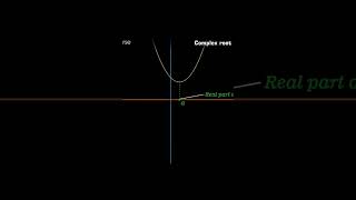
Case 3: Complex Roots (D <0)
Enroll to start learning
You’ve not yet enrolled in this course. Please enroll for free to listen to audio lessons, classroom podcasts and take practice test.
Interactive Audio Lesson
Listen to a student-teacher conversation explaining the topic in a relatable way.
Introduction to Complex Roots
🔒 Unlock Audio Lesson
Sign up and enroll to listen to this audio lesson

Today, we're going to dive into second-order homogeneous equations that lead to complex roots. Can anyone remind me what it means when we say D is less than zero?

It means the characteristic equation has no real roots, right?
Exactly! And because of this, our roots will be complex and in the form of α ± iβ. What do you think this means for the solutions?

I think that means the solutions will involve oscillations?
Great observation! The solutions indeed represent oscillatory motion. Let's delve into how we formulate the general solution for these cases.
General Solution Formulation
🔒 Unlock Audio Lesson
Sign up and enroll to listen to this audio lesson

When we have complex roots, the general solution is y(x) = e^(αx)(C cos(βx) + C sin(βx)). Who can explain what each part signifies?

The e^(αx) part shows how the amplitude changes, and the cos(βx) and sin(βx) parts show oscillations.
Exactly! The e^(αx) indicates growth or decay of the oscillations. Now, what does 'C' represent?

C is a constant that depends on initial conditions, right?
Correct! The 'C' values will be determined based on the specific initial or boundary conditions you have for your problem.
Illustrative Example
🔒 Unlock Audio Lesson
Sign up and enroll to listen to this audio lesson
Let’s consider the example y′′ + 2y′ + 5y = 0. Can someone help me identify the characteristic equation?
It would be r^2 + 2r + 5 = 0.
That's right! And what do we get when we solve this equation?
The roots are -1 ± 2i, which means we have complex roots.
Exactly! So how would we write the general solution for this case?
It would be y(x) = e^(-x)(C cos(2x) + C sin(2x)).
Well done! This solution indicates damped oscillations, which is significant in engineering.
Applications of Complex Roots
🔒 Unlock Audio Lesson
Sign up and enroll to listen to this audio lesson
Now, why do you think understanding complex roots is vital for engineers?
Because many engineering systems experience oscillations, especially during vibrations.
Exactly! For instance, in structural dynamics, knowing how systems oscillate can help in designing buildings and bridges that withstand seismic activity. Any examples you can think of?
Maybe the response of a bridge during an earthquake?
That's a perfect example! By analyzing the damped oscillations, engineers can make informed decisions to improve structural integrity.
Introduction & Overview
Read summaries of the section's main ideas at different levels of detail.
Quick Overview
Standard
In this section, we focus on the case of second-order homogeneous linear differential equations where the discriminant is less than zero, leading to complex roots. The solutions represent damped oscillations relevant to various engineering scenarios such as vibration analysis. We explore the general form of the solution, provide illustrative examples, and highlight the importance of complex roots in modeling real-world phenomena.
Detailed
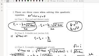
In this section, we explore second-order homogeneous linear differential equations characterized by complex roots, defined by a discriminant (D) less than zero (D < 0). When the characteristic equation yields complex conjugate roots of the form r = α ± iβ, the general solution can be expressed as:
y(x) = e^(αx)(C cos(βx) + C sin(βx))
This solution signifies oscillatory motion, often subject to exponential decay, a common characteristic of damped oscillations prevalent in engineering fields such as structural analysis and vibration science. The discussion includes an illustrative example to demonstrate the solution steps, highlighting the relevance of complex roots in modeling behaviors of mechanical systems, notably in civil engineering contexts.
Youtube Videos


Audio Book
Dive deep into the subject with an immersive audiobook experience.
Introduction to Complex Roots
Chapter 1 of 4
🔒 Unlock Audio Chapter
Sign up and enroll to access the full audio experience
Chapter Content
Let the roots be complex: r = α ± iβ
Detailed Explanation
In the context of second-order homogeneous differential equations, complex roots occur when the discriminant (D) is less than zero (D < 0). This signifies that the equation does not yield distinct real roots, which changes the nature of the solutions significantly. Instead of yielding straightforward exponential functions, complex roots introduce oscillatory behavior into the solutions.
Examples & Analogies
Imagine a swing (oscillator) that moves back and forth. When the swing is pushed gently, it moves in regular oscillations. Complex roots in differential equations can be thought of as describing how things like vibrations work in engineering, where instead of moving in a straight line, structures might sway back and forth.
General Solution for Complex Roots
Chapter 2 of 4
🔒 Unlock Audio Chapter
Sign up and enroll to access the full audio experience
Chapter Content
General Solution:
y(x) = e^αx (C cos(βx) + C sin(βx))
Detailed Explanation
The solution format for equations with complex roots incorporates both exponential and trigonometric functions. The term 'e^αx' represents an exponential function that dictates the growth or decay of the overall solution, while the terms 'C cos(βx)' and 'C sin(βx)' represent oscillations. This reflects that under certain conditions, structures will not just react instantaneously but will also show oscillatory motion over time.
Examples & Analogies
Consider a building during an earthquake. The building doesn’t just sway left and right; it has a natural frequency at which it oscillates. The general solution captures both the gradual change in the amplitude (from the exponential part) and the oscillatory nature (from the sine and cosine parts), much like how the building would sway as the forces fluctuate.
Damped Oscillations
Chapter 3 of 4
🔒 Unlock Audio Chapter
Sign up and enroll to access the full audio experience
Chapter Content
This represents damped oscillations—highly relevant in civil engineering (e.g., vibration analysis, seismic behavior).
Detailed Explanation
Damped oscillations refer to the situation where the amplitude of oscillation decreases over time due to an external force, such as friction or resistance from the environment. In civil engineering, understanding damped oscillations is crucial when designing structures that can withstand vibrations from earthquakes or wind, as it affects the stability and safety of buildings.
Examples & Analogies
Think of how a swing gradually comes to rest over time when air resistance slows it down. In engineering, if a building sways during an earthquake, dampers are often installed to reduce the swing amplitude over time, ensuring that the structure remains stable. The principles of damped oscillation help engineers create resilient designs.
Example of Solving Complex Roots
Chapter 4 of 4
🔒 Unlock Audio Chapter
Sign up and enroll to access the full audio experience
Chapter Content
Example:
y′′ + 2y′ + 5y = 0 ⇒ r² + 2r + 5 = 0 ⇒ r = −1 ± 2i
⇒ y(x) = e^(−x)(C cos(2x) + C sin(2x))
Detailed Explanation
This example shows how to connect the characteristic equation to the general solution for complex roots. The roots are calculated from the characteristic equation, which gives us r = −1 ± 2i. The negative real part (−1) implies decay in amplitude, while the imaginary part (±2i) introduces oscillation. Thus, our final general solution clearly reflects these attributes.
Examples & Analogies
This is similar to tuning a musical instrument. If the tension is too tight or loose (analogous to the real part of the roots), the pitch changes, while oscillating produces the sound waves or vibrations we hear (related to the imaginary part). The overall sound diminishes over time, showing how different elements interact just like in structural dynamics.
Key Concepts
-
Complex Roots: Roots expressed as α ± iβ arise when the discriminant is less than zero.
-
Damped Oscillations: Solutions involving exponential decay multiplied by sine and cosine functions indicate damped behaviors in systems.
-
Characteristic Equation: A vital step leading to determining the nature of roots which influences the form of the solution.
Examples & Applications
Example: Solve the equation y'' + 2y' + 5y = 0, yielding roots -1 ± 2i, leading to the general solution y(x) = e^(-x)(C cos(2x) + C sin(2x)).
Application Example: Damped oscillations in buildings during earthquakes can be analyzed using second-order differential equations with complex roots.
Memory Aids
Interactive tools to help you remember key concepts
Rhymes
Complex roots in equations do spin, oscillations rise and fall within.
Stories
Imagine a bridge shaking during an earthquake, where engineers kneel and calculate the oscillating wave over the years, creating a resilient structure.
Memory Tools
Damped OS: D for Decay, O for Oscillate, S for Solution to memorize the behavior.
Acronyms
COSINE
for Complex
for Oscillation
for Solution
for Iteration
for Numerical
for Engineering.
Flash Cards
Glossary
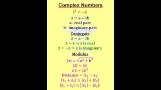
- Complex Roots
Roots of a polynomial that have both real and imaginary parts, often arising when the discriminant is negative.
- Damped Oscillations
Oscillatory motions that decrease in amplitude over time, typical in systems experiencing resistance such as friction or material damping.
- Characteristic Equation
A polynomial equation derived from a differential equation used to find its roots and hence the general solution.
Reference links
Supplementary resources to enhance your learning experience.