
Second-Order Homogeneous Equations with Constant Coefficients
Enroll to start learning
You’ve not yet enrolled in this course. Please enroll for free to listen to audio lessons, classroom podcasts and take practice test.
Interactive Audio Lesson
Listen to a student-teacher conversation explaining the topic in a relatable way.
General Form of Second-Order Homogeneous Equations
🔒 Unlock Audio Lesson
Sign up and enroll to listen to this audio lesson

Good morning, everyone! Today, we're diving into second-order homogeneous equations with constant coefficients. Can anyone remind me what a second-order equation is?

Is it an equation that involves the second derivative of a function?
Exactly, Student_1! More specifically, it can be expressed as \(\frac{d^2y}{dx^2} + b\frac{dy}{dx} + cy = 0\). This is crucial in engineering for modeling various physical phenomena. What do we mean when we say the equation is homogeneous?

It means the right-hand side is equal to zero, right?
That's correct! Remember, this homogeneity is key in simplifying our analysis. Now, why do you think knowing the constants \( a, b, c \) is important?

They help us find the specific solutions for different contexts!
Well put! The constants significantly influence the behavior of the solutions we derive.
Characteristic Equation
🔒 Unlock Audio Lesson
Sign up and enroll to listen to this audio lesson

Now, let's talk about how to solve our differential equation. We assume solutions of the form \( y = e^{rx} \). What happens when we substitute this into the original differential equation?

We end up with something like \( ar^2 + br + c = 0 \)?
Exactly, Student_4! This quadratic equation is called the characteristic equation. The roots of this equation determine the form of our general solution. Can anyone tell me the types of roots we might encounter?
We could have distinct real roots, repeated roots, or complex roots.
Perfect! Each type gives rise to a specific form of the general solution. Let’s move to how we categorize these roots.
Cases Based on Nature of Roots
🔒 Unlock Audio Lesson
Sign up and enroll to listen to this audio lesson
We just discussed the roots. Let's break them down. Who can explain what we do when we have distinct real roots?
If the discriminant is greater than zero, we get two distinct real roots, leading us to the solution \( y(x) = C_1 e^{r_1 x} + C_2 e^{r_2 x} \).
Spot on! And what about repeated real roots?
In that case, we have one root, so the form becomes \( y(x) = (C_1 + C_2 x)e^{r x}.\)
Exactly. Now, what do we learn from complex roots?
Complex roots mean oscillatory behavior, right? The solution involves sine and cosine terms.
Well done, everyone! Understanding these distinctions is vital for engineering applications.
Applications in Civil Engineering
🔒 Unlock Audio Lesson
Sign up and enroll to listen to this audio lesson
Now that we've covered the theoretical aspects, let's explore some applications, shall we? Who can name a real-world application for these equations?
The vibration of structures, like bridges or buildings!
Absolutely! The behavior during vibrations can be modeled effectively using these equations. Any other examples?
We also use them in groundwater flow problems, especially under steady-state conditions.
Correct! These equations model flow behavior accurately without needing complex simulations. Why do you think engineers need to derive unique solutions?
To ensure stability and safety in structures!
Yes, understanding behavior under different conditions is pivotal in civil engineering.
Methodical Approach to Solving
🔒 Unlock Audio Lesson
Sign up and enroll to listen to this audio lesson
Finally, let’s discuss a systematic approach to solving these equations. Can anyone outline the key steps?
First, write the differential equation in standard form.
Correct! What’s the next step?
Formulate the characteristic equation.
Right! And then?
Find the roots using the quadratic formula.
Good! What follows after finding the roots?
You write the general solution based on the nature of the roots.
Exactly! Lastly, apply any initial or boundary conditions. Great job summarizing the method, folks!
Introduction & Overview
Read summaries of the section's main ideas at different levels of detail.
Quick Overview
Standard
The section discusses the general form of second-order homogeneous linear equations with constant coefficients and provides methods for solving these equations, including determining the nature of roots. Various applications in civil engineering contexts are also highlighted.
Detailed
Detailed Summary
Second-order homogeneous equations with constant coefficients are critical in mathematical modeling for diverse fields such as civil engineering, particularly in analyzing structures, fluid dynamics, and vibrations. The general form of such an equation is expressed as:
$$\frac{d^2y}{dx^2} + b\frac{dy}{dx} + cy = 0$$
where \( a, b, c \) are real constants and \( y(x) \) is the unknown function. This equation's characteristic equation is established by substituting a solution of the form \( y = e^{rx} \), leading to a quadratic equation: $$ar^2 + br + c = 0$$. The nature of the roots of this characteristic equation dictates the general solution:
- Distinct Real Roots (D > 0): The general solution takes the form \( y(x) = C_1 e^{r_1 x} + C_2 e^{r_2 x} \).
- Repeated Real Roots (D = 0): In this case, the solution is given by \( y(x) = (C_1 + C_2 x)e^{r x} \).
- Complex Roots (D < 0): The solution involves oscillatory terms: \( y(x) = e^{\alpha x}(C_1 \cos(\beta x) + C_2 \sin(\beta x)) \).
The solutions can be applied in contexts such as free vibrations of structures, deflections of beams, and groundwater flow modeling. To establish unique solutions, initial or boundary conditions must be applied. Furthermore, a systematic approach to solving such equations is outlined, ensuring clarity in steps from forming the characteristic equation to applying the conditions for constants derived from the general solutions.
Youtube Videos


Audio Book
Dive deep into the subject with an immersive audiobook experience.
General Form of the Equation
Chapter 1 of 4
🔒 Unlock Audio Chapter
Sign up and enroll to access the full audio experience
Chapter Content
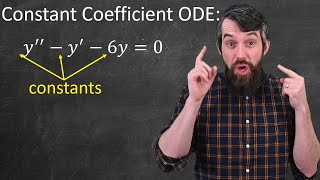
A second-order homogeneous linear differential equation with constant coefficients takes the form:
a d²y + b dy + c y = 0
dx² dx
Where:
• a,b,c are constants (real numbers),
• y(x) is the unknown function,
• d²y is the second derivative,
dx²
• The equation is homogeneous because the right-hand side is zero.
This type of equation models many real-world phenomena, such as:
• Vibrations in beams (Euler-Bernoulli beam theory),
• Free oscillations of structures,
• Groundwater flow under steady-state conditions.
Detailed Explanation
A second-order homogeneous linear differential equation with constant coefficients is represented in a standard form where the highest derivative is the second derivative (d²y/dx²). The equation is set to equal zero, indicating that it is homogeneous. The constants 'a', 'b', and 'c' are real numbers that indicate the coefficients for the respective derivatives and the unknown function 'y(x)'. Examples of situations where such equations are applicable include the analysis of vibrations in beams (like in buildings and bridges), the oscillation of mechanical structures, and the steady flow of groundwater. Each of these can be expressed with a similar second-order differential equation, making this concept crucial to various engineering problems.
Examples & Analogies
Think of a swing in a park. When you push a swing, it oscillates back and forth. The motion of the swing can be described by a second-order differential equation that captures how its position changes with time. Just like the swing's movement can be predicted, engineers use these equations to understand and predict how structures respond to forces such as wind or earthquakes.
Characteristic Equation
Chapter 2 of 4
🔒 Unlock Audio Chapter
Sign up and enroll to access the full audio experience
Chapter Content
To solve the differential equation, we assume a solution of the form:
y = e^(rx)
Substituting into the original equation:
a r² e^(rx) + b r e^(rx) + c e^(rx) = 0
Divide through by e^(rx) (never zero):
a r² + b r + c = 0
This is known as the characteristic equation or auxiliary equation.
Detailed Explanation
In order to find the solution of the second-order differential equation, we start by assuming a solution that has an exponential form, y = e^(rx). By substituting this assumed solution into the original differential equation, we can derive a simpler equation involving only the constants 'a', 'b', and 'c' and the unknown 'r', known as the characteristic equation. This characteristic equation is a quadratic equation (ar² + br + c = 0) and its roots will help determine the form of the general solution for the differential equation.
Examples & Analogies
Imagine you're trying to figure out the pattern of how a sprinter runs a straight track. You set a formula that describes their speed over time. By substituting values (like how fast the sprinter initially is) into your formula, you simplify it to find critical values. Similarly, in the characteristic equation, we simplify to find 'r', which helps us understand the underlying pattern of the system we are analyzing.
Cases Based on Nature of Roots
Chapter 3 of 4
🔒 Unlock Audio Chapter
Sign up and enroll to access the full audio experience
Chapter Content
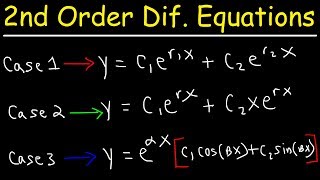
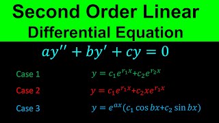
The nature of the roots determines the general solution.
Case 1: Distinct Real Roots (D = b² − 4ac > 0)
Let the roots be r₁ and r₂, with r₁ ≠ r₂ and both real.
General Solution:
y(x) = C₁ e^(r₁x) + C₂ e^(r₂x)
Case 2: Repeated Real Roots (D = 0)
Let the root be r₁ = r₂ = r.
General Solution:
y(x) = (C₁ + C₂ x) e^(r x)
Case 3: Complex Roots (D < 0)
Let the roots be complex: r₁ = α ± iβ.
General Solution:
y(x) = e^(αx)(C₁ cos(βx) + C₂ sin(βx))
Detailed Explanation
The solutions to the differential equation depend on the roots obtained from the characteristic equation. There are three primary cases based on the nature of these roots: (1) Distinct Real Roots: Here, the formula gives two different roots leading to an exponential solution based on the two roots; (2) Repeated Real Roots: This occurs when there is only one distinct root resulting in a solution with a polynomial term multiplied by an exponential function; (3) Complex Roots: This case arises when the roots have an imaginary part, and the solution incorporates sine and cosine functions which represent oscillatory motion. Each case significantly affects the behavior of the solutions in real-world scenarios.
Examples & Analogies
Picture tuning a guitar. When the strings are at the right tension (distinct roots), you hear clear notes (exponential growth). If a string is too loose or too tight (repeated roots), it produces the same note but with a different resonance. With complex tuning, the string vibrates in a specific oscillating pattern, creating harmonious sounds over time. Thus, depending on the tuning (roots), the guitar (system) behaves differently.
Applications in Civil Engineering
Chapter 4 of 4
🔒 Unlock Audio Chapter
Sign up and enroll to access the full audio experience
Chapter Content
- Free Vibration of Structures
In modeling free vibrations of a mass-spring system or cantilever beam:
d²y dy
m + c + k y = 0
dt² dt
Where:
• m: mass
• c: damping coefficient
• k: stiffness
This is a second-order homogeneous ODE. Its solution tells us whether the structure oscillates, settles, or diverges over time.
- Deflection of Beams (Euler-Bernoulli Beam Theory)
Governing equation:
d⁴y
EI = q(x)
dx⁴
For constant load q(x) = 0, this reduces to:
d⁴y = 0 ⇒ Integrating twice leads to second-order ODEs.
- Groundwater Flow (Steady-State)
Laplace's equation in 1D steady-state flow:
d²h = 0
dx²
Again, this is a homogeneous second-order equation with real constant coefficients.
Detailed Explanation
The applications of second-order homogeneous equations are vivid in civil engineering and various physical systems. The equations help model the free vibrations of structures, where mass-spring systems or beams can be analyzed for their dynamic behavior under different forces. For beam deflections, they help engineers predict how structures will deform under loads, which is essential for safety and design. Lastly, in groundwater flow under steady conditions, these equations assist in describing water behavior in soil and rock, which is vital for understanding aquifer dynamics and managing water resources.
Examples & Analogies
Consider a tall building during a storm. Engineers use these equations to model how the building will sway (free vibration) and ensure it remains safe. Similarly, think about how a playground seesaws — it must be designed not only to move freely but to return to its original position after kids have played. So, just like predicting and ensuring fun on the seesaw, we use these equations to predict the safety and stability of structures in real-world applications.
Key Concepts
-
General Form: The equation is expressed as a second-order linear equation with zero on the right side.
-
Characteristic Equation: A quadratic formed from the differential equation that helps find the roots.
-
Types of Roots: Distinct, repeated, and complex roots contribute to different general solutions.
Examples & Applications
For the equation \( y'' - 5y' + 6y = 0 \), find the characteristic equation and derive the general solution.
In the equation for free vibrations, relate the second order ODE to its physical implications in structural engineering.
Memory Aids
Interactive tools to help you remember key concepts
Rhymes
If roots are distinct, growth is quick; if repeated, they stick, in shapes that we pick.
Stories
Imagine a bridge swaying in the wind. When its vibrations follow distinct patterns, it holds strong, but if the vibrations become a single note, it might sway too much around the same point.
Memory Tools
RDC: Remember D's Character! (Roots, Discriminant, Characteristic equation)
Acronyms
ECO
Exponential for Complex Oscillation.
Flash Cards
Glossary
- Homogeneous Equation
An equation where the right-hand side is equal to zero.
- Characteristic Equation
A quadratic equation derived from the substitution of potential solutions into the original differential equation.
- Distinct Real Roots
Two different real solutions obtained from the characteristic equation.
- Repeated Real Roots
The situation where the characteristic equation yields a single real solution with multiplicity.
- Complex Roots
Solutions of the characteristic equation that exist as conjugate pairs, involving imaginary components.
- General Solution
The complete solution of the homogeneous equation expressed in terms of arbitrary constants.
Reference links
Supplementary resources to enhance your learning experience.