
Methodical Approach to Solving Second-Order Homogeneous Equations
Enroll to start learning
You’ve not yet enrolled in this course. Please enroll for free to listen to audio lessons, classroom podcasts and take practice test.
Interactive Audio Lesson
Listen to a student-teacher conversation explaining the topic in a relatable way.
Understanding the Differential Equation
🔒 Unlock Audio Lesson
Sign up and enroll to listen to this audio lesson

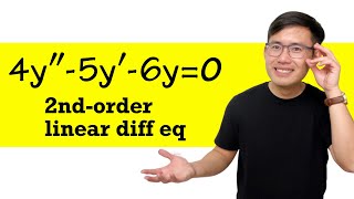
Can someone tell me what form the second-order homogeneous differential equation takes?

It’s something like d²y/dx² + b dy/dx + c y = 0.
Exactly! So, what does each term represent?

The coefficients a, b, and c are constants, right?
Correct. And what does it mean for the right-hand side to be zero?

That means the equation is homogeneous!
Right! Remember, *homogeneous* means no external source term.
Let's summarize: the equation has constant coefficients and indeed models many real phenomena.
Forming the Characteristic Equation
🔒 Unlock Audio Lesson
Sign up and enroll to listen to this audio lesson

After identifying the differential equation, what’s our next step?
We form the characteristic equation: ar² + br + c = 0.
Exactly! What do we assume for solutions of the equation?

We assume solutions of the form y = e^(rx).
Correct again! Substituting that in gives us the roots. How do we find these roots?
We use the quadratic formula!
Great! Always remember the quadratic formula can help find r, our roots!
Let's wrap up: we've formed the characteristic equation, which directs our next steps.
Analyzing the Roots
🔒 Unlock Audio Lesson
Sign up and enroll to listen to this audio lesson
Now that we have our roots, how do we determine their nature?
We check the discriminant, D, right? D = b² - 4ac?
Absolutely! What do the resulting values signify?
If D > 0, we have distinct real roots.
And if D = 0, we have repeated real roots.
If D < 0, we get complex roots!
Exactly right! The roots tell us how the system behaves: oscillatory, exponential growth or decay. Summarize this understanding in your notes!
Writing the General Solution
🔒 Unlock Audio Lesson
Sign up and enroll to listen to this audio lesson
Now we must write the general solution. What form does it take based on the root types?
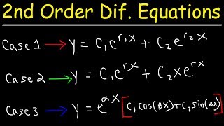
For distinct real roots, it’s C₁e^(r₁x) + C₂e^(r₂x).
Correct! What about repeated roots?
That one is (C₁ + C₂x)e^(r₁x) since we have an additional x for the polynomial.
And for complex roots?
It's e^(αx)(C₁cos(βx) + C₂sin(βx)).
Perfect! Different roots generate different forms of solutions!
Applying Initial Conditions
🔒 Unlock Audio Lesson
Sign up and enroll to listen to this audio lesson
Finally, how do we use the initial conditions to find C₁ and C₂?
We substitute the initial values into the general solution.
And we solve the resulting equations, right?
Exactly! This step is crucial for specifying the solution to meet given conditions.
Are these constants always the same?
Not at all! They'll vary with different initial conditions. Great job! Let's recap our six steps!
Introduction & Overview
Read summaries of the section's main ideas at different levels of detail.
Quick Overview
Standard
The section details a methodical process for addressing second-order homogeneous differential equations by formulating the characteristic equation, determining root types, writing general solutions, and applying initial conditions, providing clarity and thoroughness in the problem-solving approach.
Detailed
Methodical Approach to Solving Second-Order Homogeneous Equations
This section succinctly outlines a six-step strategy aimed at creating efficiency in solving second-order homogeneous linear differential equations with constant coefficients.
Step 1: Write the Differential Equation
Ensure the equation is expressed in the standard form:
$$\frac{d^2y}{dx^2} + b\frac{dy}{dx} + cy = 0$$
Step 2: Form the Characteristic Equation
Translate the original differential equation into its characteristic form, formulated as:
$$ar^2 + br + c = 0$$
Step 3: Find the Roots
Utilize the quadratic formula to solve for the roots:
$$r = \frac{-b \pm \sqrt{b^2 - 4ac}}{2a}$$
Step 4: Determine the Type of Roots
Identify if the roots are distinct real numbers, real and equal, or complex conjugates, as these dictate the next steps in solution forms.
Step 5: Write the General Solution Based on Root Type
Revisit Section 3.3 for the corresponding structures of the solutions depending on the nature of the roots derived.
Step 6: Apply Initial/Boundary Conditions
Use specific provided values of y(x_0) and y'(x_0) to evaluate C_1 and C_2 to hone in on a unique solution.
This systematic approach not only augments comprehension but also equips engineers and mathematicians with the skills to efficiently solve differential equations encountered in practical applications.
Youtube Videos


Audio Book
Dive deep into the subject with an immersive audiobook experience.
Step 1: Write the Differential Equation
Chapter 1 of 6
🔒 Unlock Audio Chapter
Sign up and enroll to access the full audio experience
Chapter Content
Ensure it's in the standard form:
d2y
dy
a + b + cy = 0
dx2
dx
Detailed Explanation
The first step in solving second-order homogeneous equations is to write the differential equation in standard form. In this form, the equation is represented as a combination of the second derivative, the first derivative, and the function itself, all set equal to zero. This structure is crucial because it indicates that the equation is homogeneous (there is no term that is just a constant or function of independent variables). Ensure that you identify the constants a, b, and c correctly from your equation.
Examples & Analogies
Think of this step as setting the stage before a performance. Just like you need to have the scenery and props in place before the actors start, you need to have the equation in its correct form before you start solving it.
Step 2: Form the Characteristic Equation
Chapter 2 of 6
🔒 Unlock Audio Chapter
Sign up and enroll to access the full audio experience
Chapter Content
Form the characteristic equation:
ar2 + br + c = 0
Detailed Explanation
In the second step, you form the characteristic equation from the standard differential equation. This is achieved by assuming a solution of the form y = e^(rx) and substituting it into the original differential equation. After simplification, you derive a quadratic equation in the form ar² + br + c = 0, which is essential for finding the roots of the differential equation.
Examples & Analogies
Imagine you're building a bridge. The characteristic equation is like the blueprint of the bridge—without it, you wouldn’t know how to proceed with building the actual structure.
Step 3: Find the Roots
Chapter 3 of 6
🔒 Unlock Audio Chapter
Sign up and enroll to access the full audio experience
Chapter Content
Use the quadratic formula:
√
−b ± √(b²−4ac)
r = 2a
Detailed Explanation
The next step involves finding the roots of the characteristic equation using the quadratic formula. The roots (r) will help determine the general solution of the differential equation. By substituting the coefficients a, b, and c into the formula, you can find the nature of the roots which will dictate the form of your solution in later steps.
Examples & Analogies
Finding the roots is like solving a mystery—each clue (the coefficients a, b, and c) helps you uncover the truth about the behavior of the system you are studying.
Step 4: Determine the Type of Roots
Chapter 4 of 6
🔒 Unlock Audio Chapter
Sign up and enroll to access the full audio experience
Chapter Content
• Real and distinct
• Real and equal
• Complex conjugate
Detailed Explanation
In this step, you categorize the roots you've found into three types: real and distinct, real and equal, or complex conjugates. Understanding the type of roots is crucial because each type leads to a different form of the general solution for the differential equation. The discriminant (D = b² - 4ac) plays a key role in determining the nature of the roots.
Examples & Analogies
Think of this step as sorting fruits. Just as apples, oranges, and bananas each require different storage conditions, the different types of roots indicate different solutions that must be treated in specific ways.
Step 5: Write the General Solution Based on Root Type
Chapter 5 of 6
🔒 Unlock Audio Chapter
Sign up and enroll to access the full audio experience
Chapter Content
Refer to Section 3.3 for the structure of the solution.
Detailed Explanation
After determining the type of roots, the next step is to write the general solution based on that classification. For real distinct roots, the solution takes the form y(x) = C₁e^(r₁x) + C₂e^(r₂x). If the roots are repeated, you'll have a solution of y(x) = (C₁ + C₂x)e^(rx). In the case of complex roots, it evolves into y(x) = e^(αx)(C₁cos(βx) + C₂sin(βx)). Each form is tailored to the nature of the roots, reflecting the behavior of the system.
Examples & Analogies
Writing the general solution is like cooking according to a recipe—different ingredients (type of roots) will yield different final dishes (solutions) based on your recipe (formulas for general solutions).
Step 6: Apply Initial/Boundary Conditions
Chapter 6 of 6
🔒 Unlock Audio Chapter
Sign up and enroll to access the full audio experience
Chapter Content
Use given values of y(x₀) and y′(x₀) to solve for constants C₁, C₂.
Detailed Explanation
The final step involves applying any initial or boundary conditions provided in the problem to find the specific values of the constants C₁ and C₂ in your general solution. This step is fundamental for obtaining a unique solution that corresponds to the physical situation being modeled. Substitute the initial values into your general solution to solve for these constants effectively.
Examples & Analogies
This step is like tailoring a suit. Just as a tailor adjusts the fit based on the specific measurements of the customer, applying initial or boundary conditions customizes the general solution to fit the particular problem at hand.
Key Concepts
-
Characteristic Equation: A quadratic equation formed from the coefficients of the differential equation.
-
Roots: Values derived from the characteristic equation that influence the general solution form.
-
Homogeneous Differential Equation: An equation that equates to zero with no persistent external terms.
-
General Solution: A comprehensive solution of the differential equation characterized by constants determined from initial conditions.
Examples & Applications
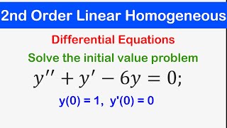
Example of solving d²y/dx² - 4y = 0 leads to y(x) = C₁e^(2x) + C₂e^(-2x).
Application of initial conditions in y(0) = 1, y'(0) = 0 to determine specific constants for a unique solution.
Memory Aids
Interactive tools to help you remember key concepts
Rhymes
Roots that are real make solutions ideal, if they’re complex, oscillations appear as we peal.
Stories
Imagine a bridge oscillating in a storm. If roots are real, it stands still; if complex, it dances to the wind’s Will.
Memory Tools
To remember the steps: Write, Form, Find, Determine, Write (solution), Apply — 'WFF D W'
Acronyms
R.E.A.D. for the roots! Real, Equal, or complex
R.E.A.D. tells the tale of where we next step.
Flash Cards
Glossary
- Characteristic Equation
The quadratic equation derived from a second-order differential equation, represented as ar² + br + c = 0.
- Homogeneous Equation
A differential equation where all terms depend only on the function and its derivatives, equating to zero.
- Roots
The values of r from the characteristic equation that inform the form of the general solution.
- General Solution
The solution of a differential equation expressed with arbitrary constants, contingent upon specific initial conditions.
- Discriminant
A value computed as D = b² - 4ac in the characteristic equation, determining the nature of the roots.
Reference links
Supplementary resources to enhance your learning experience.