
Smith Chart Design
Interactive Audio Lesson
Listen to a student-teacher conversation explaining the topic in a relatable way.
Normalization of Impedance
🔒 Unlock Audio Lesson
Sign up and enroll to listen to this audio lesson

Today, we're going to discuss the crucial first step in using the Smith Chart: normalizing impedance. Can anyone tell me why we normalize impedances?

Isn't it to make the calculations easier by referencing it to a standard?
Exactly! So, to normalize an impedance, we use the formula: z_L = Z_L/Z_0, where Z_0 is the characteristic impedance of our system. This allows us to plot on the Smith Chart. What do you think is our next step after normalization?

We plot the normalized impedance on the Smith Chart?
That's correct! Once we plot z_L on the chart, we can begin our journey toward finding the right matching components.

Can you explain again how to calculate normalized impedance?
Certainly! Just divide the load impedance by the reference impedance: z_L = Z_L/Z_0. For instance, if we have Z_L as 75Ω and Z_0 as 50Ω, we would calculate it as 75/50 = 1.5. Remembering this process helps streamline our matching designs.

Got it! So, we normalize to 1.5 before plotting.
Exactly! This is the first step towards using the Smith Chart effectively.
Plotting on the Smith Chart
🔒 Unlock Audio Lesson
Sign up and enroll to listen to this audio lesson

Now that we’ve normalized our impedance, let’s discuss how we actually plot this on the Smith Chart. Who can remind us what type of point we mark on the chart?
Is it the normalized load impedance?
That’s right! We place the point corresponding to our normalized z_L onto the Smith Chart grid. What comes after that?
We follow the circles for Γ?
Yes! We navigate through the constant Γ circles. These represent our reflection coefficients. Why do you think following these circles is important?
To visualize how adding components affects our matching?
Correct! By moving along these circles, we can understand how to add series or shunt components to reach a perfect impedance match.
Example of Smith Chart Design
🔒 Unlock Audio Lesson
Sign up and enroll to listen to this audio lesson
Let’s put our knowledge to the test with a practical example. We want to match a 50Ω source to a 75Ω load using the Smith Chart. Who can tell me the first step?
We need to normalize the 75Ω load impedance.
Exactly! So, we calculate z_L as 75Ω/50Ω, which equals 1.5. Now, what do we do with this value?
We plot it on the Smith Chart.
Good! Next, we need to decide what type of components, inductors or capacitors, we will use. Does anyone recall how we determine this?
By observing the distance on the chart to see if we need to go toward inductive or capacitive components?
Correct! After plotting, we found that to go from 1.5 to a full match, we need a series inductor and a shunt capacitor. Let’s calculate their values.
Introduction & Overview
Read summaries of the section's main ideas at different levels of detail.
Quick Overview
Standard
The Smith Chart is a vital tool for designing matching networks. It visualizes normalized impedances and allows engineers to follow constant reflection coefficient circles to achieve impedance matching. The section details key steps in using the chart, including normalizing impedance and plotting. An example illustrates practical application.
Detailed
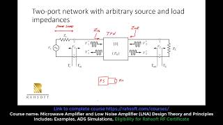
The Smith Chart is a powerful tool in RF engineering used for impedance matching, and it presents a complex plane where impedances can be visualized and manipulated. This section outlines crucial steps for using the Smith Chart effectively, beginning with the normalization of the load impedance relative to the characteristic impedance of the transmission line. Once normalized, the load impedance is plotted on the Smith Chart, where engineers can navigate through constant reflection coefficient (Γ) circles to visualize the effects of adding series or shunt reactive components (inductors or capacitors) in order to achieve a perfect match. The section also provides a practical example of matching a 50Ω source to a 75Ω load using series inductors and shunt capacitors at a frequency of 1GHz. This approach enables the efficient transfer of power by minimizing reflections and optimizing bandwidth.
Youtube Videos


Audio Book
Dive deep into the subject with an immersive audiobook experience.
Key Steps in Smith Chart Design
Chapter 1 of 2
🔒 Unlock Audio Chapter
Sign up and enroll to access the full audio experience
Chapter Content
10.3.1 Key Steps:
- Normalize Impedance:
\[ z_L = \frac{Z_L}{Z_0} \]
2. Plot \( z_L \) on Smith Chart.
3. Follow Constant \( Γ \) Circles:
- Series L/C: Move along constant resistance circles.
- Shunt L/C: Move along constant conductance circles.
Detailed Explanation
In the process of designing using the Smith Chart, the first step is to normalize the impedance. Normalization means converting the load impedance (Z_L) to a unitless value (z_L) by dividing it by a known reference impedance (Z_0). This makes it easier to plot on the chart.
Next, you plot z_L on the Smith Chart. The Smith Chart is a specialized graph that helps visualize complex impedance transformations. After plotting, the designer needs to follow specific circles on the chart. For a series inductor or capacitor, you move along constant resistance circles. For shunt reactive components, movement is along constant conductance circles. This helps in identifying the required component values that enable matching to the desired impedance.
Examples & Analogies
Imagine the Smith Chart as a map for traveling through a complex city. First, you need to figure out where you are (normalize your impedance) before navigating to your destination (matching impedance). As you drive (plotting on the chart), you must follow certain paths (constant circles) to get to your goal, whether it's to a coffee shop (series L/C) or a park (shunt L/C).
Example of Smith Chart Design
Chapter 2 of 2
🔒 Unlock Audio Chapter
Sign up and enroll to access the full audio experience
Chapter Content
10.3.2 Example (50Ω → 75Ω Match):
- Solution:
- Series Inductor: \( L = 6.5 \text{nH} \) at 1GHz.
- Shunt Capacitor: \( C = 2.1 \text{pF} \) at 1GHz.
Detailed Explanation
In a practical example of using a Smith Chart to design a matching network, we want to match an impedance from 50 ohms (Ω) to 75 Ω. This involves analyzing the positions on the Smith Chart to determine the values of the necessary components. Based on the calculations from the Smith Chart, a series inductor of 6.5 nanohenries (nH) and a shunt capacitor of 2.1 picofarads (pF) are required, and this is specifically for operation at a frequency of 1 GHz.
Examples & Analogies
Think of this example like adjusting the settings on your home stereo system to match the acoustics of your room. You might need to add a subwoofer (the inductor) to balance the bass and a tweeter (the capacitor) to enhance the high frequencies, ensuring everything sounds just right in your specific space (matching the load impedance).
Key Concepts
-
Normalization of Impedance: A process that adjusts impedance values to a standard reference for analyzing on the Smith Chart.
-
Plotting on the Smith Chart: The act of marking normalized impedance on the Smith Chart for further analysis.
-
Constant Γ Circles: Visual elements on the Smith Chart that help determine how to add components for impedance matching.
Examples & Applications
To match a 50Ω source with a 75Ω load, first normalize by calculating z_L = 75Ω/50Ω = 1.5.
When plotting normalized impedance of 1.5 on the Smith Chart, you can observe the subsequent movement along constant Γ circles to determine required inductive or capacitive components.
Memory Aids
Interactive tools to help you remember key concepts
Rhymes
To match the load, we take a step, Normalize the value, be sure to prep!
Stories
Imagine a race where impedances need to align perfectly to achieve full power transfer. The Smith Chart is like the racecourse guiding them to the finish line where power flows seamlessly.
Memory Tools
N-P-C: Normalize, Plot, Circle! The steps you follow on the Smith Chart.
Acronyms
P.L.A.C.E
Plot Load
Add Components
End with matching!
Flash Cards
Glossary
- Smith Chart
A graphical tool used in RF engineering for impedance matching and visualization of complex impedances.
- Normalized Impedance
Impedance values scaled to a reference standard (Z0) for easier analysis on the Smith Chart.
- Reflection Coefficient (Γ)
A parameter that describes how much of a wave is reflected by an impedance discontinuity in the transmission line.
- Constant Γ Circles
Curves on the Smith Chart representing locations where the reflection coefficient is constant.
Reference links
Supplementary resources to enhance your learning experience.