
Two-Port Network Design - Matching Networks
Interactive Audio Lesson
Listen to a student-teacher conversation explaining the topic in a relatable way.
Introduction to Impedance Matching
🔒 Unlock Audio Lesson
Sign up and enroll to listen to this audio lesson

Today, we're going to discuss impedance matching. The central goal is maximizing power transfer between the source and the load. Can anyone tell me why this is important?

It reduces signal reflections, right?
Exactly! Reflections can cause interference. This can be represented with the reflection coefficient, Γ. It's calculated using this formula: Γ = (Z_L - Z_S*) / (Z_L + Z_S).

What do you mean by Z_L and Z_S?
Good question! Z_L represents the load impedance, and Z_S is the source impedance. When we achieve Γ = 0, it means we have a perfect match, and the VSWR is 1. Does anyone know what VSWR stands for?

It stands for Voltage Standing Wave Ratio!
Great! Remember, the lower the VSWR, the better the match.
To summarize, impedance matching maximizes power transfer, reduces reflections, and is quantified by reflection coefficients and VSWR.
L-Section Matching and its Design
🔒 Unlock Audio Lesson
Sign up and enroll to listen to this audio lesson

Next, let's look at the L-section matching network. Who can describe the topology of an L-section?

It's a simple arrangement with either a capacitor or an inductor between the source and the load.
Correct! Depending on whether the load resistance is greater or less than the source resistance, we can derive specific design equations. Student_1, can you share the equations for when R_L is greater than R_S?
Sure! When R_L > R_S, we use X_L = sqrt{R_L(R_L - R_S)}, and X_C = (R_S R_L) / X_L.
Exactly! And what about when R_L is less than R_S?
Then we use X_C = sqrt{R_S(R_S - R_L)}, and X_L = (R_S R_L) / X_C.
Great work! L-section matching is fundamental for RF applications. Can anyone think of scenarios where we would specifically use L-sections?
For low-frequency applications or audio circuitry!
Absolutely right! Remember, L-sections are quite versatile, but they can be limited in bandwidth.
So far, we covered L-section networks, constructing them based on the resistance relationships and where they are utilized.
Smith Chart and its Use
🔒 Unlock Audio Lesson
Sign up and enroll to listen to this audio lesson
Now, let's delve into the Smith Chart. Who has heard of it before?
I've seen it, but I'm not sure how to use it.
No worries! The Smith Chart helps with impedance matching visually. First, we normalize the load impedance. Can anyone remind us how to do that?
We use z_L = Z_L / Z_0.
Correct! After that, we plot z_L on the chart and follow the constant Γ circles. If we want to move towards a match, what do we do?
We follow the resistance circles for series components.
And for shunt components, we follow constant conductance circles, right?
Exactly! Understanding this will help us amend mismatches effectively. Let’s practice plotting some example impedances on the Smith Chart.
Transmission Line Matching Techniques
🔒 Unlock Audio Lesson
Sign up and enroll to listen to this audio lesson
Moving on, let’s focus on transmission line matching using techniques like quarter-wave transformers. Can anyone describe what a quarter-wave transformer does?
It transforms one impedance to another using a specific length of transmission line?
That’s right! The formula for its transformation is Z_1 = sqrt{Z_0 * Z_L}. Can someone calculate Z_1 if we have Z_0 = 50Ω and Z_L = 100Ω?
Z_1 would be about 70.7Ω!
Exactly! And what about single-stub matching? What does it involve?
Using an open or short stub at a distance to cancel reactance?
Exactly, fantastic! Remember too that the length of the stub plays a crucial role. Let's summarize: we learned about quarter-wave transformers and single-stub matching, crucial for efficient impedance transformation in RF designs.
Broadband Matching Techniques
🔒 Unlock Audio Lesson
Sign up and enroll to listen to this audio lesson
Finally, let's examine broadband matching techniques, like multi-section matching and tapered lines. Who can explain what Chebyshev response means in this context?
It allows us to minimize reflections over a wider bandwidth!
Exactly! Multi-section matching can achieve this, along with tapered lines. Can anyone recall how the exponential taper formula looks?
It’s Z(z) = Z_0 * e^{αz}.
Correct! Such techniques are particularly useful in systems requiring consistent performance over a broad frequency range. To conclude our lesson: effective broadband matching is essential for high-performance circuits.
Introduction & Overview
Read summaries of the section's main ideas at different levels of detail.
Quick Overview
Standard
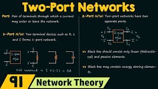
Impedance matching is crucial for maximizing power transfer and minimizing reflections in two-port networks. This section outlines different matching network topologies such as L-sections, Pi, and T networks, along with methods like quarter-wave transformers and broadband matching techniques. It provides design equations, practical examples, and highlights key practical considerations.
Detailed
Detailed Summary
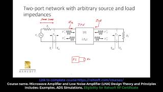
In this section, we explore the critical concept of impedance matching in two-port networks, primarily focusing on the significance of maximizing power transfer and reducing signal reflections. The core objective is described mathematically using the reflection coefficient (Γ) and voltage standing wave ratio (VSWR), where a perfect match is achieved when Γ equals zero.
Matching Network Topologies
Different matching network designs are discussed:
1. L-Section Matching: A simple topology using either inductors or capacitors to match impedances based on the source and load resistances, employing specific design equations.
2. Pi (π) and T-Networks: These topologies, suitable for high-Q and low-impedance applications, utilize combinations of inductors and capacitors to achieve better matching.
Smith Chart Design
The Smith Chart is introduced as a graphical tool for impedance matching, showcasing the normalization of impedances and the use of constant Γ circles for series and shunt components.
Transmission Line Matching Techniques
Quarter-wave transformers and single-stub matching are techniques outlined for impedance transformation and reactance cancellation, respectively, along with practical design examples.
Broadband Matching
Multi-section matching and tapered lines allow for improved performance over a broader bandwidth by controlling reflections and optimizing power transfer efficiently.
Practical Considerations
Considerations such as component losses and PCB layout effects are highlighted, emphasizing the importance of effective design.Q factors and parasitic elements that influence overall performance are discussed.
Through comprehensive examples and summarizing tables, this section offers an essential overview for understanding matching networks in electronic design.
Youtube Videos

Audio Book
Dive deep into the subject with an immersive audiobook experience.
Introduction to Impedance Matching
Chapter 1 of 15
🔒 Unlock Audio Chapter
Sign up and enroll to access the full audio experience
Chapter Content
10.1 Introduction to Impedance Matching
- Objective:
- Maximize power transfer between source and load by eliminating reflections.
- Key Concepts:
- Reflection Coefficient (Γ):
\[
Γ = \frac{Z_L - Z_S^*}{Z_L + Z_S}
\] - VSWR (Voltage Standing Wave Ratio):
\[
VSWR = \frac{1 + |Γ|}{1 - |Γ|}
\] - Perfect Match: \( Γ = 0 \), \( VSWR = 1 \).
Detailed Explanation
Impedance matching is crucial in ensuring that maximum power is transferred between the source (like a generator) and the load (like an antenna or speaker). When reflection occurs, some of the power sent from the source bounces back instead of being absorbed by the load. This is quantified using the Reflection Coefficient (Γ). It tells us how much power is reflected back. A perfect match occurs when Γ is zero, meaning all the power is transmitted,
leading to a VSWR of 1, indicating no reflections.
Examples & Analogies
Imagine you are trying to pour water from a pitcher into a cup. If the cup is too small or positioned improperly, some water will spill out, similar to how power gets reflected if there’s a mismatched impedance. A perfect match is like having the pitcher perfectly aligned over the cup where all the water goes in, meaning all the power is efficiently transferred.
Matching Network Topologies: L-Section Matching
Chapter 2 of 15
🔒 Unlock Audio Chapter
Sign up and enroll to access the full audio experience
Chapter Content
10.2 Matching Network Topologies
10.2.1 L-Section Matching
- Topology:
Source ──┬── L/C ── Load
│
C/L
- Design Equations:
- For \( R_L > R_S \):
\[
X_L = \sqrt{R_L(R_L - R_S)}, \quad X_C = \frac{R_S R_L}{X_L}
\] - For \( R_L < R_S \):
\[
X_C = \sqrt{R_S(R_S - R_L)}, \quad X_L = \frac{R_S R_L}{X_C}
\]
Detailed Explanation
The L-section matching network consists of either an inductor (L) or a capacitor (C) connected between the source and load. Depending on the relative sizes of the source resistance (R_S) and load resistance (R_L), the network can be designed with either an inductor or a capacitor for matching. The provided equations help calculate the reactance values required for different scenarios so that impedance matches and power transfer is optimized.
Examples & Analogies
Think of the L-section matching network like an adjustable wrench used to fit different sized nuts. If the bolt is too big, you tighten the wrench (like adding reactance with an inductor). If it’s too small, you loosen it up (adding reactance with a capacitor). In both cases, you’re making sure the wrench works perfectly with the bolt, just like a matching network ensures the source and load work well together.
Matching Network Topologies: Pi (π) and T-Networks
Chapter 3 of 15
🔒 Unlock Audio Chapter
Sign up and enroll to access the full audio experience
Chapter Content
10.2.2 Pi (π) and T-Networks
- Pi-Network:
Source ──┬── C1 ──┬── Load
│ │
L C2
│ │
GND GND
- Used for high-Q matching (e.g., RF amplifiers).
- T-Network:
Source ── L1 ──┬── L2 ── Load
│
C
│
GND
- Better for low-impedance loads.
Detailed Explanation
The Pi and T networks represent two common topologies for matching networks. The Pi-network offers better performance for high-Q (Quality factor) applications, such as RF amplifiers, where precise impedance matching is essential for efficient operation. The T-network, on the other hand, is often employed with low-impedance loads, allowing flexibility in adjusting the matching conditions effectively while maintaining stability.
Examples & Analogies
Consider a road network analogy. A Pi-network can be like a roundabout where traffic flows seamlessly, minimizing stops (losses), essential for high-speed areas (like RF). In contrast, a T-network resembles a series of stoplights that allow control over traffic but might be more suitable for areas with lower speeds, ensuring everything flows correctly with lower impedance.
Smith Chart Design: Key Steps
Chapter 4 of 15
🔒 Unlock Audio Chapter
Sign up and enroll to access the full audio experience
Chapter Content
10.3 Smith Chart Design
10.3.1 Key Steps:
- Normalize Impedance:
\[
z_L = \frac{Z_L}{Z_0}
\] - Plot \( z_L \) on Smith Chart.
- Follow Constant \( Γ \) Circles:
- Series L/C: Move along constant resistance circles.
- Shunt L/C: Move along constant conductance circles.
Detailed Explanation
Using a Smith Chart is a graphical method to solve matching problems. The first step involves normalizing the load impedance to a reference impedance (Z_0, often 50Ω or 75Ω). After normalizing, you plot this point on the Smith Chart. The next steps involve visually navigating the chart along constant Γ circles to determine the necessary components for achieving an impedance match, whether by adding series or shunt reactances.
Examples & Analogies
Using a Smith Chart can be likened to navigating through a city using a map. The normalized impedance serves as your starting point, while the constant Γ circles guide your route to the correct matching components, similar to finding the best path on a map to reach your destination efficiently.
Example of Smith Chart Design (50Ω → 75Ω Match)
Chapter 5 of 15
🔒 Unlock Audio Chapter
Sign up and enroll to access the full audio experience
Chapter Content
10.3.2 Example (50Ω → 75Ω Match):
- Solution:
- Series Inductor: \( L = 6.5 \text{nH} \) at 1GHz.
- Shunt Capacitor: \( C = 2.1 \text{pF} \) at 1GHz.
Detailed Explanation
This example demonstrates how to match an impedance from 50Ω to 75Ω using the Smith Chart. By following the key steps outlined before, it’s found that placing a series inductor of 6.5 nH and a shunt capacitor of 2.1 pF at a frequency of 1 GHz achieves the required impedance transformation for optimal power transfer.
Examples & Analogies
Picture a sports team adjusting its strategy for a specific opponent. The series inductor (like a defensive player) protects against specific plays of the opposing team (the mismatch), while the shunt capacitor (like a strategic offense) helps score by making adjustments on the fly to ensure both sides work together for success on the field.
Transmission Line Matching: Quarter-Wave Transformer
Chapter 6 of 15
🔒 Unlock Audio Chapter
Sign up and enroll to access the full audio experience
Chapter Content
10.4 Transmission Line Matching
10.4.1 Quarter-Wave Transformer
- Impedance Transformation:
\[
Z_1 = \sqrt{Z_0 Z_L}
\] - Example: Match 50Ω to 100Ω:
\[
Z_1 = \sqrt{50 \times 100} ≈ 70.7Ω
\]
Detailed Explanation
A quarter-wave transformer is another matching technique that utilizes a specific length of transmission line to transform impedances between a source and load. The length is a quarter of the wavelength of the signal being transmitted. By calculating the square root of the product of the source impedance (Z_0) and load impedance (Z_L), you can find the required impedance of the transformer (Z_1) to ensure an efficient match.
Examples & Analogies
Imagine tuning a piano. A quarter-wave transformer is like adjusting the tension of a string to hit the right note. Matching the tension (impedance) ensures that the sound produced is rich and full, just like matching impedances ensures the signal is transmitted without loss.
Transmission Line Matching: Single-Stub Matching
Chapter 7 of 15
🔒 Unlock Audio Chapter
Sign up and enroll to access the full audio experience
Chapter Content
10.4.2 Single-Stub Matching
- Shunt Stub:
Source ──λ/4──┬── Load
│
Stub (Open/Short)
- Design: Adjust stub length to cancel reactance.
Detailed Explanation
Single-stub matching involves using an additional reactive component (the stub) connected to a transmission line. The key to this matching technique is adjusting the length of the stub to effectively cancel out the reactive component of the load impedance, allowing for a pure resistive match. This helps in minimizing reflections and maximizing power transfer.
Examples & Analogies
Think of single-stub matching like gardening, where you adjust the height of different plants to create a visually balanced arrangement. By adjusting the stub length (like pruning the plants), you're ensuring that everything fits and works harmoniously together, minimizing any 'garden clutter' (reflections) in the process.
Broadband Matching: Multi-Section Matching
Chapter 8 of 15
🔒 Unlock Audio Chapter
Sign up and enroll to access the full audio experience
Chapter Content
10.5 Broadband Matching
10.5.1 Multi-Section Matching
- Chebyshev Response:
- Minimizes reflections over a wide bandwidth.
Detailed Explanation
Multi-section matching utilizes multiple reactive components in a more complex configuration that can handle a broader range of frequencies. The Chebyshev response is designed to achieve low reflection coefficients across a wide bandwidth, allowing the system to maintain performance even as frequencies vary.
Examples & Analogies
Consider a multi-section matching network like a well-organized toolbox, where each tool (component) is designed for a specific purpose. Just as having the right tool for various tasks ensures efficiency, having multiple components for different frequencies ensures maximal performance across a wider spectrum.
Broadband Matching: Tapered Lines
Chapter 9 of 15
🔒 Unlock Audio Chapter
Sign up and enroll to access the full audio experience
Chapter Content
10.5.2 Tapered Lines
- Exponential Taper:
\[
Z(z) = Z_0 e^{αz}
\]
Detailed Explanation
Tapered lines are used in broadband matching to gradually transition the impedance from one level to another. By varying the width of the transmission line, the impedance can change smoothly, minimizing reflections and optimizing power transfer across a wider frequency range. The exponential taper function allows for precise control over this impedance transition.
Examples & Analogies
Just like a ramp allows smooth transitions for wheelchairs, tapered lines provide a gradual change in impedance. This ensures signals move from one area to another seamlessly without abrupt changes that might cause signal losses, much like providing a smooth path makes the journey easier.
Practical Considerations: Component Losses
Chapter 10 of 15
🔒 Unlock Audio Chapter
Sign up and enroll to access the full audio experience
Chapter Content
10.6 Practical Considerations
10.6.1 Component Losses
- Effective Q-Factor:
\[
Q_{eff} = \frac{f_0}{BW} \leq \frac{1}{2} \sqrt{\frac{R_{high}}{R_{low}} - 1}
\]
Detailed Explanation
The effective Q-factor measures the quality of a resonant circuit. It is influenced by losses in the components used. The formula provided establishes a relationship between the resonant frequency (f_0), bandwidth (BW), and the ratio of resistances in the network. Understanding and optimizing the Q-factor can help improve performance.
Examples & Analogies
Think of the Q-factor as the efficiency of a car engine. A high Q-factor means the engine runs smoothly with little wasted energy, while a low Q-factor indicates more losses. By optimizing the components (like tuning an engine), you can maximize efficiency and performance.
Practical Considerations: PCB Layout Effects
Chapter 11 of 15
🔒 Unlock Audio Chapter
Sign up and enroll to access the full audio experience
Chapter Content
10.6.2 PCB Layout Effects
- Parasitics:
- Trace inductance (~1nH/mm).
- Pad capacitance (~0.1pF).
Detailed Explanation
PCB (Printed Circuit Board) layout plays a significant role in the effectiveness of matching networks. Parasitic elements, such as inductance and capacitance in traces and pads, introduce unexpected behavior in the circuit, which can negatively impact performance. Understanding these effects is vital to designing efficient matching networks.
Examples & Analogies
Consider laying track for a train. If the tracks are not aligned properly (like poorly designed PCB traces), the train (signal) can derail or slow down. Proper PCB layout ensures that signals travel smoothly without interference from parasitics, just like well-laid tracks keep a train running efficiently.
Lab Experiment: L-Network Matching Setup
Chapter 12 of 15
🔒 Unlock Audio Chapter
Sign up and enroll to access the full audio experience
Chapter Content
10.7 Lab Experiment: L-Network Matching
10.7.1 Setup:
- VNA (Vector Network Analyzer).
- DUT: 50Ω source → 100Ω load.
Detailed Explanation
In this lab experiment, a Vector Network Analyzer (VNA) is utilized to measure the performance of an L-network used to match a 50Ω source with a 100Ω load. The setup allows the analysis of how effectively the matching circuit enhances power transfer and reduces reflections.
Examples & Analogies
Running this experiment is like using a thermometer to check the temperature of food. You want to determine if it's cooked just right (properly matched) or if it needs more time or adjustments to ensure the meal is perfect (optimal power transfer).
Lab Experiment: Measurements
Chapter 13 of 15
🔒 Unlock Audio Chapter
Sign up and enroll to access the full audio experience
Chapter Content
10.7.2 Measurements:
- Without Matching:
- \( Γ ≈ 0.33 \), \( VSWR ≈ 2.0 \).
- With L-Network:
- \( Γ < 0.05 \), \( VSWR ≈ 1.1 \).
Detailed Explanation
The measurements show the impact of impedance matching. Without the matching network, the Reflection Coefficient (Γ) is approximately 0.33, indicating significant power loss back to the source, observed with a VSWR of 2.0. After implementing the L-network, Γ drops below 0.05, showing virtually all power is being used, reflected in a VSWR close to 1.1, representing effective matching.
Examples & Analogies
Think of this as measuring the efficiency of a water faucet. When it’s tangled with kinks (mismatches), water (power) sprays everywhere, wasting it. After fixing the hose with a proper connection (matching network), the flow becomes smooth, ensuring that almost all water goes into the glass, ideal just like the minimized reflections in the experiment.
Summary Table of Matching Methods
Chapter 14 of 15
🔒 Unlock Audio Chapter
Sign up and enroll to access the full audio experience
Chapter Content
10.8 Summary Table
| Matching Method | Bandwidth | Complexity | Typical Use |
|---|---|---|---|
| L-Section | Narrow | Low | DC-100MHz |
| π/T-Network | Medium | Medium | RF (1MHz-2GHz) |
| λ/4 Transformer | Narrow | Low | Microwave |
| Stub Matching | Medium | High | >500MHz |
| Multi-Stage | Wide | Very High | Broadband Systems |
Detailed Explanation
This table summarizes different matching methods, their bandwidth capabilities, complexity, and typical applications. The methods range from simple L-sections suitable for low-frequency applications to complex multi-stage matching systems designed for broadband use. Each method’s effectiveness varies with application requirements and frequency range.
Examples & Analogies
Imagine different types of Swiss Army knives suited for specific tasks. Some are straightforward, like the L-section method for simple jobs, while others are more complex, equipped with multiple tools (multi-stage matching) for diverse uses. Knowing which tool to choose based on the task's demands ensures efficiency.
Key Equations for Matching Networks
Chapter 15 of 15
🔒 Unlock Audio Chapter
Sign up and enroll to access the full audio experience
Chapter Content
10.9 Key Equations
- L-Section Components:
\[
Q = \sqrt{\frac{R_{high}}{R_{low}} - 1}
\] - Stub Length (Open-Circuit):
\[
l = \frac{λ}{2π} \tan^{-1}\left(\frac{B}{Y_0}\right)
\]
Detailed Explanation
These key equations offer essential calculations for designing matching networks. The first equation gives the quality factor (Q) in relation to the effective resistances encountered. The second equation describes how to determine the length of an open-circuit stub based on its impedance and frequency. Mastering these equations is critical for optimizing matching networks.
Examples & Analogies
Understanding these equations is akin to having a recipe for a dish. The first equation provides a way to gauge the quality of ingredients (resistances), while the second helps determine the right amount of each ingredient (stub length) needed to achieve the perfect taste (matching).
Key Concepts
-
Impedance Matching: Essential for maximizing power transfer and minimizing reflections in RF systems.
-
Reflection Coefficient (Γ): Measures the proportion of the signal that is reflected back, affecting performance.
-
VSWR: A critical parameter indicating the efficiency of power transfer from source to load.
-
L-Section Matching: A straightforward topology used for basic impedance matching.
-
Broadband Matching: Techniques designed to enhance performance across a wider frequency spectrum.
Examples & Applications
Example of an L-Network adjusting 50Ω to match a 100Ω load using capacitors and inductors.
Calculating the quarter-wave transformer design parameters to match a 50Ω system to a 100Ω load.
Memory Aids
Interactive tools to help you remember key concepts
Rhymes
Power transfer's the name of the game, zero reflections are our aim.
Stories
Imagine a water pipe network; when the pipes connect smoothly, no water leaks out, maximizing flow, much like impedance matching in electrical circuits.
Memory Tools
Remember 'Γ = (Z_L - Z_S) / (Z_L + Z_S)', where G stands for Gain in power; it reflects how well we transmit signals!
Acronyms
For VSWR, think 'Very Smooth Wave Routing' to remind you that a low VSWR means efficient line matching.
Flash Cards
Glossary
- Impedance Matching
The process of making the impedance of a source match that of the load to maximize power transfer.
- Reflection Coefficient (Γ)
A measure of how much power is reflected back from the load.
- VSWR (Voltage Standing Wave Ratio)
A measure of how effectively radio frequency power is transmitted from the power source to the load.
- LSection
A basic matching network configuration using an inductor or capacitor.
- Pi Network
A matching network configuration shaped like the Greek letter π, includes two capacitors and one inductor.
- TNetwork
A matching network arrangement that resembles the letter T, useful for low-impedance applications.
- Smith Chart
A graphical representation used for impedance matching.
- QuarterWave Transformer
A transmission line used to transform impedances by λ/4 length.
- Stub Matching
A technique that uses a short transmission line segment for reactive compensation.
- Broadband Matching
Techniques used to minimize reflections over a wide range of frequencies.
Reference links
Supplementary resources to enhance your learning experience.