
Analog Electronic Circuits
Enroll to start learning
You’ve not yet enrolled in this course. Please enroll for free to listen to audio lessons, classroom podcasts and take practice test.
Interactive Audio Lesson
Listen to a student-teacher conversation explaining the topic in a relatable way.
Introduction to the Common Source Amplifier
🔒 Unlock Audio Lesson
Sign up and enroll to listen to this audio lesson

Today, we will discuss the Common Source Amplifier, a fundamental configuration in analog electronics. Can anyone tell me what they think a common source amplifier does?

I think it amplifies voltage signals, right?
Exactly! The Common Source Amplifier is known for its ability to amplify voltage. Now, what's an important phase when analyzing these amplifiers?

Setting the DC bias to zero?
Correct! By setting the DC bias to zero, we simplify the analysis to focus on small signals. Let’s dive into the small signal equivalent circuit next.
Voltage Gain Calculation
🔒 Unlock Audio Lesson
Sign up and enroll to listen to this audio lesson

The voltage gain of a Common Source Amplifier is defined as A = -RD * gm. Can someone explain what RD and gm represent?

RD is the drain resistance, and gm is the transconductance of the transistor.
Well done! Now, if RD is 3k ohms and gm is 2mA/V, what would the voltage gain be?

It would be A = -3k * 2mA/V = -6.
Exactly! The gain is -6. Remember that the negative sign indicates a phase reversal. Let's explore the output resistance next.
Output and Input Resistance
🔒 Unlock Audio Lesson
Sign up and enroll to listen to this audio lesson
What can you tell me about the output resistance of our amplifier?
I think the output resistance is just the drain resistance, RD.
That’s correct! The output resistance RO is equal to RD. What about the input resistance?
Isn't the input resistance supposed to be very high because the gate current is zero?
Absolutely! The input resistance is considered infinite in ideal conditions. This makes it suitable for voltage amplification. Let’s summarize our discussion.
Today, we covered the basics of the Common Source Amplifier, including voltage gain, output, and input resistance.
High Frequency Effects
🔒 Unlock Audio Lesson
Sign up and enroll to listen to this audio lesson
Now let’s talk about high frequency scenarios. Why is it important to consider parasitic capacitances?
Because they can affect the signal integrity and gain?
Exactly! Specifically, Cgs and Cgd can influence our amplifier's behavior. What tool can we use to analyze the impact of these capacitances?
Miller's theorem helps us translate these capacitances into an equivalent capacitance.
Great! Understanding these effects is vital for designing stable and effective amplifiers. Let’s review what we’ve learned so far.
Introduction & Overview
Read summaries of the section's main ideas at different levels of detail.
Quick Overview
Standard
In this section, we explore the Common Source Amplifier's small signal equivalent circuit, emphasizing the significance of setting the DC bias to zero. Key calculations for voltage gain, output resistance, and input resistance are derived, alongside discussions on various operational conditions including high-frequency effects.
Detailed
Detailed Summary
Common Source Amplifier Overview
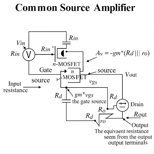
The Common Source Amplifier is a fundamental configuration in analog electronics, primarily used for amplifying voltage signals. In analyzing its small signal equivalent circuit, we simplify the circuit by setting the DC bias conditions to zero, allowing for linear behavior in response to small input voltages.
Key Parameters
- Voltage Gain (A): The voltage gain is defined as the ratio of the small signal output voltage to the small signal input voltage, denoted as A = -RD * gm, where RD is the drain resistance and gm is the transconductance of the transistor.
- Output Resistance (RO): The output resistance can be determined by looking into the output port. It is calculated as RO = RD, assuming ideal conditions where the input is driven to an AC ground.
- Input Resistance (Rin): The input resistance of the amplifier is ideally infinite as no DC current flows into the gate terminal during small signal analysis. Rin is calculated as the parallel combination of resistors at the input.
High Frequency Considerations
In high frequency scenarios, parasitic capacitances can significantly impact the amplifier's performance. This includes gate-to-source capacitance (Cgs) and gate-to-drain capacitance (Cgd), which can be analyzed using Miller's theorem to determine the effective capacitance seen from the input terminal.
Conclusion
The Common Source Amplifier, despite its lower voltage gain compared to other configurations like the common emitter amplifier, plays a critical role in MOSFET-based designs, especially in microelectronics and VLSI applications. Understanding its behavior under different conditions, including biasing and frequency effects, is essential for effective circuit design.
Youtube Videos

Audio Book
Dive deep into the subject with an immersive audiobook experience.
Introduction to Common Source Amplifier
Chapter 1 of 8
🔒 Unlock Audio Chapter
Sign up and enroll to access the full audio experience
Chapter Content
Welcome back after the short break and we are about to start the small signal equivalent circuit for the Common Source Amplifier.
Detailed Explanation
This section introduces the topic of the Common Source Amplifier. After a brief break, the lecture shifts focus to small signal equivalent circuits, which are a crucial aspect in understanding how amplifiers operate under varying input conditions. The small signal model simplifies the analysis by focusing only on the fluctuations around a specific operating point, instead of the entire nonlinear behavior of the circuit.
Examples & Analogies
Imagine driving a car. When you're cruising at a steady speed, small accelerations or decelerations are akin to the small signal variations in an amplifier. Just as you'd focus on the small adjustments to maintain speed, engineers focus on small signal models to examine how amplifiers respond to tiny changes in input.
Setting DC Bias to Zero
Chapter 2 of 8
🔒 Unlock Audio Chapter
Sign up and enroll to access the full audio experience
Chapter Content
In the small signal equivalent circuit first thing is that we are making the DC bias to be 0.
Detailed Explanation
Setting the DC bias to zero implies that any DC component in the signal is ignored when analyzing small signal behavior. This is important as it allows the circuit analysis to concentrate solely on the variations that are superimposed on the DC levels. By doing this, the small signal model becomes linear and easier to work with mathematically.
Examples & Analogies
Consider a seesaw that is initially balanced. By setting the DC bias to zero, we can focus only on the minor adjustments that individuals make to either end of the seesaw, instead of considering its original balanced position.
Understanding Small Signal Parameters
Chapter 3 of 8
🔒 Unlock Audio Chapter
Sign up and enroll to access the full audio experience
Chapter Content
The linearity is defined by this gm. So, the expression of the i it is given here, this part is the gm as I was telling before or we can have another expression of the gm here.
Detailed Explanation
In small signal analysis, the parameter 'gm' is the transconductance, which defines how much the output current changes in response to a small change in input voltage. This parameter is crucial for determining the gain of the amplifier. The discussion highlights the relationship between input signal variations (vgs) and output current fluctuations (i), establishing the foundational relationship for amplifier operation.
Examples & Analogies
Think of gm like the sensitivity of a dimmer switch for lights. A slight twist on the knob (input voltage) will cause a noticeable change in brightness (output current/voltage). The more sensitive the switch (higher gm), the more effective it is at controlling brightness with small adjustments.
Voltage Gain Calculation
Chapter 4 of 8
🔒 Unlock Audio Chapter
Sign up and enroll to access the full audio experience
Chapter Content
So, that gives us the voltage gain A defined as vout/vs = -RD×gm.
Detailed Explanation
The voltage gain (A) of the Common Source Amplifier can be expressed as a ratio of output voltage (vout) to input voltage (vs). This specific gain formula highlights the dependence of the output signal on both the drain resistance (RD) and the transconductance (gm), indicating that increasing either can improve the amplification effect. The negative sign indicates that the output is inverted relative to the input.
Examples & Analogies
Imagine a megaphone where the input is your voice, and the louder the input, the louder the output will be for the audience. Here, RD is like the speaker’s volume capability — more powerful speakers can project your voice louder (higher gain), while the inversion means that what you say (input) comes out reversed.
Output Resistance Consideration
Chapter 5 of 8
🔒 Unlock Audio Chapter
Sign up and enroll to access the full audio experience
Chapter Content
The second parameter it is the output resistance.
Detailed Explanation
Output resistance is a vital parameter for amplifiers, as it affects how the amplifier interacts with the load connected to it. In analyzing the circuit, if we observe the output resistance when connected to a signal source, we can determine how much of the input signal is impeded by the internal characteristics of the circuit. This impacts overall performance and efficiency for the signals being amplified.
Examples & Analogies
Consider a water hose connected to a fountain. The resistance of the hose affects how much water flows out (output resistance). If the hose is too thin or blocked, less water will flow, similar to how low output resistance can restrict output signals.
Input Side Resistance Analysis
Chapter 6 of 8
🔒 Unlock Audio Chapter
Sign up and enroll to access the full audio experience
Chapter Content
Now, the third parameter it is; so, at the input port if we see and if you see what is the corresponding resistance here.
Detailed Explanation
The input resistance is crucial for understanding how much input signal the amplifier can accept without drawing too much current. By analyzing this resistance, we can ensure that the amplifier will minimize loading effects, preserving the integrity of the incoming signals. Thus, an optimal input resistance will allow for efficient signal transmission into the amplifier.
Examples & Analogies
Think of a high impedance input as a sponge soaking up water. If the sponge (amplifier) is too dense (low input resistance), it won't absorb water (input signal) effectively. A proper balance ensures that maximum water is soaked up without overflowing.
Common Source vs. Common Emitter
Chapter 7 of 8
🔒 Unlock Audio Chapter
Sign up and enroll to access the full audio experience
Chapter Content
We can say that performance wise common emitter amplifier it is better than the common source amplifier. So, both gain wise and the output swing wise.
Detailed Explanation
The comparison between common source amplifiers and common emitter amplifiers reveals differences in performance metrics such as gain and output swing. While common emitter amplifiers might generally provide better performance, common source amplifiers are preferred in specific applications, especially in integrated circuits and VLSI designs where MOSFETs are utilized. This highlights the trade-offs between design choices.
Examples & Analogies
Imagine choosing between two cars. One has better fuel efficiency (common emitter) but the other is built to do heavy lifting and carrying loads (common source). Depending on the job at hand, you might pick one over the other based on specific automotive features, just as engineers choose amplifiers based on intended applications.
Numerical Example and Gain Calculation
Chapter 8 of 8
🔒 Unlock Audio Chapter
Sign up and enroll to access the full audio experience
Chapter Content
So, how do you then find the gain, how do you find the gain of the circuit and or from this information.
Detailed Explanation
In the numerical example, calculations are performed using available parameters to find the circuit gain at certain operating points. By applying given values to derive the behavior of the amplifier, such as biasing and output swing, students gain practical experience in using theoretical knowledge to analyze real circuits. Understanding this process can aid in effectively designing amplifiers for practical applications.
Examples & Analogies
Consider baking a cake. You start with a recipe (theoretical knowledge) but need to measure out ingredients (circuit parameters) and follow steps carefully to ensure the cake turns out perfectly. Similarly, precise calculations help ensure circuit performance meets design expectations.
Key Concepts
-
Common Source Amplifier: A basic amplifier configuration that enhances voltage signals.
-
Voltage Gain (A): Defined based on the drain resistance and transconductance of the MOSFET.
-
Output Resistance (RO): Equal to the drain resistance and critical for load behavior.
-
Input Resistance (Rin): The input side resistance is typically infinite in ideal conditions.
-
High Frequency Effects: Involves parasitic capacitances affecting circuit behaviors.
Examples & Applications
The voltage gain of a Common Source Amplifier can be calculated as -RD * gm. For example, if RD = 3kΩ and gm = 2mA/V, the gain is -6.
For high-frequency applications, the effect of parasitic capacitances like Cgs and Cgd need to be considered to maintain signal integrity.
Memory Aids
Interactive tools to help you remember key concepts
Rhymes
For voltage gain that's a boon, remember RD and gm to tune.
Stories
Imagine a fountain (Common Source) where the water flows (input voltage) based on the hose diameter (RD) and pressure (gm).
Memory Tools
‘GIVE’ for Gain = Input Voltage * Output Voltage / R.
Acronyms
Acronym ‘GAM’ for Gain = RD * gm; Remember it as Gain from Amplifier's MOSFET.
Flash Cards
Glossary
- Common Source Amplifier
An amplifier configuration that primarily enhances voltage signals using a MOSFET.
- Voltage Gain (A)
The ratio of the output voltage to the input voltage, typically expressed as A = -RD * gm.
- Transconductance (gm)
Measures how effectively a device converts input voltage into output current.
- Output Resistance (RO)
The resistance seen by the load connected at the output, usually equivalent to the drain resistance RD.
- Input Resistance (Rin)
The resistance seen at the input terminal of the amplifier, often considered infinite.
- Parasitic Capacitance
Unwanted capacitances that arise from physical layout and can affect circuit performance.
- Miller Effect
Phenomenon where the input capacitance is modified by the amplification factor, resulting in increased effective input capacitance.
Reference links
Supplementary resources to enhance your learning experience.