
Bode Plot and Corner Frequency
Enroll to start learning
You’ve not yet enrolled in this course. Please enroll for free to listen to audio lessons, classroom podcasts and take practice test.
Interactive Audio Lesson
Listen to a student-teacher conversation explaining the topic in a relatable way.
Understanding Frequency Response in RC Circuits
🔒 Unlock Audio Lesson
Sign up and enroll to listen to this audio lesson

Good morning class! Today, we'll be discussing the frequency response of RC circuits. Can anyone remind me what we mean by frequency response?

Is it how a circuit reacts to different frequencies of input signals?
Exactly, it describes how the output signal magnitude and phase shift respond as the input frequency varies. Now, when we analyze RC circuits in the frequency domain, we often use the Bode plot. Can anyone tell me what a Bode plot is?

Isn't it a graph that shows the gain and phase shift of a circuit over a frequency range?
Yes! It represents logarithmic frequency on one axis and the magnitude in decibels on the other. Very useful for visualizing circuit behavior. Now let's examine corner frequencies and why they are important.
Corner Frequencies and Their Significance
🔒 Unlock Audio Lesson
Sign up and enroll to listen to this audio lesson

Let’s talk about corner frequencies. What can you tell me about them?

A corner frequency is where the gain begins to drop in a Bode plot, right?
Yes, nicely put! It's the frequency at which the output voltage drops to -3 dB compared to the maximum output. How does this relate to transfer functions?

The location of the pole dictates where that corner frequency occurs.
Exactly! Understanding this relationship helps us design circuits effectively. Can someone provide an example of a practical application?
It helps in setting audio equalizers to avoid feedback by managing gain at different frequencies.
Great example! It’s crucial in real-world applications.
Bode Plot Characteristics
🔒 Unlock Audio Lesson
Sign up and enroll to listen to this audio lesson
Moving on, let’s discuss the characteristics of Bode plots. Why do we express gain in decibels?
Because it compresses the scale and makes it easier to visualize large ranges of gain.
Spot on! The slope of the Bode plot provides significant information. What do we observe about gain slopes after the corner frequency?
The gain decreases at -20 dB per decade after the corner frequency.
Correct! This roll-off is essential to predict circuit behavior.
Analyzing Circuit Behavior and Implications
🔒 Unlock Audio Lesson
Sign up and enroll to listen to this audio lesson
Now let's analyze the implications of circuit behavior affected by corner frequencies. How does this relate to designing an amplifier?
We need to choose components carefully to ensure the amplifier operates within desired frequencies.
Exactly! Selecting appropriate resistors and capacitors can help achieve required corner frequencies for desired performance.
And if we know the pole locations, we can predict how the circuit will respond?
Yes! Predicting response accurately is crucial for design efficiency.
Introduction & Overview
Read summaries of the section's main ideas at different levels of detail.
Quick Overview
Standard
In this section, we delve into the frequency response of RC circuits, focusing on how Bode plots can be utilized to visualize gain and phase shift over varying frequencies. It emphasizes understanding corner frequencies and their relationship to the poles of the transfer function, providing insights into practical applications in circuit design.
Detailed
In this section, we explore the concept of frequency response in RC circuits, particularly how Bode plots provide a clear representation of circuit gain and phase shift over a range of frequencies. The discussion begins by analyzing the transfer function in the Laplace domain and replaces 's' with 'jω' for frequency domain representation. We examine how the magnitudes of output voltages in low and high frequencies behave, noting the hyperbolic nature beyond certain corner frequencies.
The significance of corner frequencies is highlighted as they relate directly to the location of poles in the transfer function, affecting circuit behavior in terms of passbands and stopbands. Key characteristics of Bode plots are introduced, illustrating that gains remain constant up to the corner frequency before rolling off at -20 dB per decade. Furthermore, we analyze the relationship between poles and cutoff frequencies, showcasing their importance in amplifier designs.
Youtube Videos

Audio Book
Dive deep into the subject with an immersive audiobook experience.
Understanding Frequency Response
Chapter 1 of 6
🔒 Unlock Audio Chapter
Sign up and enroll to access the full audio experience
Chapter Content
So, similar to the C-R circuit again here what you are doing is that we are taking the circuit into Laplace domain, namely the impedance of both the elements we are going in Laplace domain for C it is and this is directly same as this R. And then input it is V in Laplace domain s and then the corresponding output also we are considering in Laplace domain which is V (s).
Detailed Explanation
In this section, we start by converting the circuit to the Laplace domain. This involves representing the resistances and capacitances in terms of their impedances, which allows us to analyze how the circuit responds to different frequencies. In this domain, we denote the input voltage as V(in) and the output voltage as V(s). This transformation is a crucial step in analyzing the circuit's frequency response because it simplifies the mathematics involved.
Examples & Analogies
Think of converting the circuit into the Laplace domain like changing from standard time to a movie format where time is abstracted. Instead of tracking the scene minute by minute, you see the entire film (the circuit) and can easily analyze parts without always referencing back to specific timestamps (the original time domain representation).
Obtaining the Transfer Function
Chapter 2 of 6
🔒 Unlock Audio Chapter
Sign up and enroll to access the full audio experience
Chapter Content
Now, to get the frequency response as I said for the previous case what you have to do, we have to take this replace this s by jω or rather I was having say sigma part in s which I am making it 0. So, we are dropping this part and that gives us the transfer function in Fourier domain and it becomes .
Detailed Explanation
The next step involves replacing the variable 's' with 'jω' in our equation. This substitution turns our Laplace transform into a Fourier transform, which is useful for examining the steady-state frequency response of the circuit. By making this change, we can analyze how different frequencies affect the output of the circuit compared to its input.
Examples & Analogies
Imagine tuning a musical instrument: just like you adjust the pitch (frequency) to see how well it resonates, replacing 's' with 'jω' allows you to see how the circuit behaves at different frequencies, tuning into each one to understand its effect.
Gain and Phase Variation
Chapter 3 of 6
🔒 Unlock Audio Chapter
Sign up and enroll to access the full audio experience
Chapter Content
So, again here what you can do? We can plot the magnitude. So, if we consider the | | and with respect to ω. So, if you see here at low frequency; if we ignore this part with respect to 1, then the corresponding magnitude it is 1. But then if you go to higher and higher frequency and if this part it is dominating over this 1, then the magnitude wise what we will be seeing here it is 1 by ω nature.
Detailed Explanation
In this section, we discuss the behavior of the circuit's magnitude as the frequency varies. At low frequencies, the magnitude remains stable at 1 because the reactance of the capacitor is minimal. As the frequency increases, the influence of the capacitor becomes more pronounced, leading to a decrease in the output magnitude. Specifically, we can observe a change where the output behaves like '1/ω', indicating a gradual roll-off in gain as frequency increases.
Examples & Analogies
Consider how you can easily hear someone speaking at low volume (low frequency), but as the noise in a room increases (higher frequency), it becomes harder to hear them clearly. This is similar to how the circuit begins to lose signal clarity and strength (magnitude) as we increase the frequencies.
Characterizing Corner Frequency
Chapter 4 of 6
🔒 Unlock Audio Chapter
Sign up and enroll to access the full audio experience
Chapter Content
So, I should say if I call this is ω at ω RC = 1 which means ω = . So, if I consider the actual curve instead of considering this two asymptotic or approximated curve will be getting the actual curve going like this. So, here again, it is having complementary behavior as I said with respect to the previous one.
Detailed Explanation
The corner frequency, also called the cutoff frequency, is defined where the behavior of the circuit transitions. Specifically, it is where the reactance of the capacitor equals the resistance, resulting in ωRC = 1. At this frequency, the gain begins to drop significantly, and we can observe the circuit transitioning from passing signals effectively to attenuating them.
Examples & Analogies
Think of the corner frequency like a threshold in a race. Below this threshold speed (frequency), runners (signals) can move freely with minimal resistance. But as they approach and exceed that point, obstacles start emerging (the circuit becomes reactive), which significantly slows their progress (attenuates the signal).
Visualizing with Bode Plot
Chapter 5 of 6
🔒 Unlock Audio Chapter
Sign up and enroll to access the full audio experience
Chapter Content
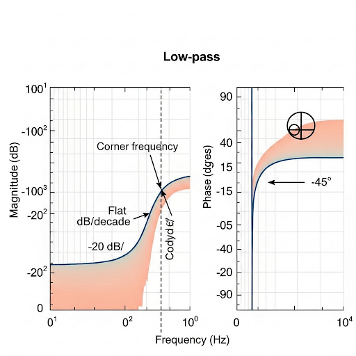
So, whatever we get is the Bode plot. So, here again in the Bode plot what will be seen it is similar to the previous case that if you consider ω in log scale then of course, 0 frequency it will be pushed to ∞ distance and then this hyperbolic part on the other hand, it will be having a linear behavior.
Detailed Explanation
The Bode plot is a graphical representation of the gain and phase of the circuit's frequency response on a logarithmic scale. It effectively shows how the circuit behaves across a wide range of frequencies. Here, the gain starts at 0 dB and then varies with frequency in a linear fashion. This plot is crucial for engineers to easily observe stability, gain margins, and behavior around the corner frequency.
Examples & Analogies
Imagine you are charting your progress on a fitness journey: instead of measuring every single step, you sum your total progress at regular intervals (like looking at gains over weeks on a log scale). The Bode plot does the same by summarizing the frequency responses of the circuit over broader intervals, making it easier to recognize patterns and important transitions.
Connecting Poles and Corner Frequency
Chapter 6 of 6
🔒 Unlock Audio Chapter
Sign up and enroll to access the full audio experience
Chapter Content
So, again here we are getting a direct relationship of this pole and this corner frequency. So, just by seeing the transfer function; if we know that the location of the pole probably from that we can tell what is the location of this corner frequency.
Detailed Explanation
This section emphasizes the relationship between the poles of the transfer function and the corner frequency. The position of poles (which reflect the system's stability and response characteristics) can directly tell us where the corner frequency lies in relation to our frequency response—allowing engineers to predict the behavior of their circuits effectively.
Examples & Analogies
Think of it like a map where every landmark's position tells you how far you are from reaching a specific destination (the corner frequency). Knowing exactly where the poles are is like having a GPS to guide you accurately to avoid confusion while navigating through various frequencies.
Key Concepts
-
Frequency Response: How output varies with input frequency.
-
Bode Plot: Visual representation of frequency response.
-
Corner Frequency: Point where gain reduces by -3 dB.
-
Poles: Locations in the transfer function affecting frequency response.
-
Gain Decay: The decrease of gain past certain frequencies, typically -20 dB/decade.
Examples & Applications
In audio systems, corner frequencies are crucial to avoid feedback and ensure clarity in sound.
Frequency response testing in amplifiers helps determine their effective operational range.
Memory Aids
Interactive tools to help you remember key concepts
Rhymes
When the frequencies play, the gain will sway; past corner points, watch it decay!
Stories
Imagine you are a sound engineer tuning an amplifier. You set the corner frequency to avoid feedback, balancing high and low tones to create clear sound. The Bode plot helps you visualize this balance!
Memory Tools
Remember 'PIG G', for 'Poles Indicate Gain's Gradual decline.'
Acronyms
CUTE for remembering Corner frequency, Unity gain, Transfer function, and Effects on behavior.
Flash Cards
Glossary
- Bode Plot
A graph that represents the gain and phase of a circuit as a function of frequency, plotted on logarithmic scales.
- Corner Frequency
The frequency at which the gain of a circuit is -3 dB from its maximum value.
- Transfer Function
A mathematical representation of the relationship between the input and output of a system in the Laplace domain.
- Pole
A value in the Laplace domain that indicates a frequency where the output response of a system decreases significantly.
- Gain
The ratio of output voltage to input voltage, often expressed in decibels.
Reference links
Supplementary resources to enhance your learning experience.