
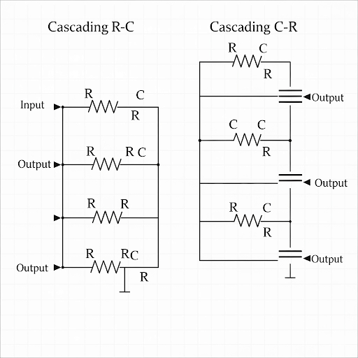
Cascading R-C and C-R circuits
Enroll to start learning
You’ve not yet enrolled in this course. Please enroll for free to listen to audio lessons, classroom podcasts and take practice test.
Interactive Audio Lesson
Listen to a student-teacher conversation explaining the topic in a relatable way.
Introduction to R-C Circuit Frequency Response
🔒 Unlock Audio Lesson
Sign up and enroll to listen to this audio lesson

Welcome everyone! Today we'll begin our journey with R-C circuits. Can anyone tell me what happens to the signal at low frequencies?

I think the capacitor acts like an open circuit, right?
Exactly! When the frequency is low, the capacitor will not conduct current, allowing the signal to pass through. This characteristic makes R-C circuits low-pass filters. Now, what do you think happens as the frequency increases?

The capacitor will start to short the output signal.
Correct! At high frequencies, the capacitor has low impedance, causing the output to drop. We can express this drop mathematically using transfer functions. How do we obtain them?
Frequency Response Representation
🔒 Unlock Audio Lesson
Sign up and enroll to listen to this audio lesson

Let’s talk about Bode plots. They combine both gain and phase perspectives. Can anyone recall how we transition from the Laplace domain to frequency representation?

By substituting `s` with `jω`!
Yes! By substituting `s` with `jω`, we get to visualize how gain behaves at different frequencies. What do we see in the gain plot as we reach the corner frequency?

It drops at -20 dB per decade after that point.
Right again! Understanding this behavior is essential for designing effective filters and amplifiers.
C-R Circuit Characteristics
🔒 Unlock Audio Lesson
Sign up and enroll to listen to this audio lesson
Having covered R-C circuits, it’s now time for C-R circuits. What’s the primary distinction between the two?
C-R circuits allow higher frequencies to pass through.
Exactly right! C-R circuits have a high-pass characteristic. What does the phase plot look like at lower frequencies?
It starts with a phase shift of +90°, right?
Correct! The shift indicates that low-frequency signals are progressively attenuated as we move up. This is crucial for designing state-of-the-art filters.
Cascading R-C and C-R Circuits
🔒 Unlock Audio Lesson
Sign up and enroll to listen to this audio lesson
Finally, let’s discuss cascading. What issues might arise when cascading R-C and C-R circuits?
Loading effects can occur, affecting the output signal.
Spot on! To mitigate these effects, we often use amplifiers. What role does an ideal voltage amplifier play in this context?
It helps ensure the previous circuit doesn't load down the next one.
Exactly! Knowing this helps us design effective multi-stage amplifiers. Remember, analyzing the overall transfer function is key!
Introduction & Overview
Read summaries of the section's main ideas at different levels of detail.
Quick Overview
Standard
The section delves into the analysis of R-C and C-R circuits in the Laplace and Fourier domains. It emphasizes the significance of poles in determining cutoff frequencies and provides a thorough understanding of gain and phase plots in both cases.
Detailed
Cascading R-C and C-R Circuits
In this section, we explore the behavior of R-C and C-R circuits when analyzed in the Laplace domain and their corresponding frequency responses in Fourier domain. Starting with R-C circuits, we derive transfer functions and discuss how replacing s with jω leads to gain and phase plots.
The frequency behavior summarizes a low-pass characteristic where the output signal passes lower frequencies efficiently but attenuates higher frequencies beyond a certain cutoff frequency, defined where the magnitude approaches 0.707 of the max output. This frequency response is typically showcased in a Bode plot, illustrating a linear decline in gain post-break frequency at a rate of -20 dB/decade.
Similarly, C-R circuits present an inverse behavior where phase shift and gain alterations occur over the frequency spectrum. Emphasis is placed on pole-zero relationships and the influence on circuit design as cascading R-C and C-R circuits interact, making the understanding of loading effects crucial to maintain performance. The section wraps up by detailing the overall implications these circuit configurations have on amplifier designs.
Youtube Videos

Audio Book
Dive deep into the subject with an immersive audiobook experience.
Understanding Impedance and Transfer Functions
Chapter 1 of 6
🔒 Unlock Audio Chapter
Sign up and enroll to access the full audio experience
Chapter Content
So, similar to the C-R circuit again here what you are doing is that we are taking the circuit into Laplace domain, namely the impedance of both the elements we are going in Laplace domain for C it is and this is directly same as this R. And then input it is V in Laplace domain s and then the corresponding output also we are considering in Laplace domain which is V (s).
And, if we analyze this circuit what you are getting here it is V (s) = . So, from that what your yeah what you are getting is = . It is similar to the previous circuit except of course, we do not have the sRC part rather in the numerator we do have simply 1.
Detailed Explanation
In this chunk, we are discussing the transition of the circuit analysis from the time domain to the Laplace domain. In the Laplace domain, we represent circuit elements like resistors and capacitors using their impedances. The voltage input (Vin) and output (V(s)) are also expressed in terms of the Laplace variable 's'. The equation represents the transfer function, which relates input and output voltage in the circuit context. The unique aspect here is that while the circuit's behavior can vary; the approach to analysis remains consistent from C-R to R-C circuits.
Examples & Analogies
Imagine a water pipe where the flow rate (voltage) is affected by the valve (resistor) and any obstructions (capacitor) in the pipe. When we discuss this in the Laplace domain, we conceptually transform the physical behaviors into a mathematical model that allows us to predict the flow rate under different conditions. This is similar to predicting a water flow based on pipe size and pressure changes.
Frequency Response Analysis
Chapter 2 of 6
🔒 Unlock Audio Chapter
Sign up and enroll to access the full audio experience
Chapter Content
Now, to get the frequency response as I said for the previous case what you have to do, we have to take this replace this s by jω or rather I was having say sigma part in s which I am making it 0. So, we are dropping this part and that gives us the transfer function in Fourier domain and it becomes. Now, this transfer function in Fourier domain again you can make the gain plot and the phase plot to get the frequency response.
Detailed Explanation
To analyze the circuit's frequency response, which is how the output signal changes with frequency, we replace 's' in the Laplace transform with 'jω', where 'j' is the imaginary unit and 'ω' is the angular frequency. This substitution allows us to convert the transfer function into the Fourier domain, making it easier to graphically represent gain and phase shifts across different frequencies through gain and phase plots.
Examples & Analogies
Think about tuning a radio. You adjust the frequency (the knob) to find a station. Similarly, in electronics, by moving through different frequencies, we observe how well the circuit responds at each frequency. The transfer function acts like a guide, showing us where the circuit is 'tuned in' for signal amplification.
Magnitude Response at Different Frequencies
Chapter 3 of 6
🔒 Unlock Audio Chapter
Sign up and enroll to access the full audio experience
Chapter Content
So, again here what you can do? We can plot the magnitude. So, if we consider the | | and with respect to ω. So, if you see here at low frequency; if we ignore this part with respect to 1, then the corresponding magnitude it is 1. But then if you go to higher and higher frequency and if this part it is dominating over this 1, then the magnitude wise what we will be seeing here it is 1 by ω nature.
Detailed Explanation
In this analysis, we investigate how the circuit's output magnitude reacts as we vary the frequency ω. At low frequencies, the output closely resembles the input, resulting in a gain of 1. However, as we increase the frequency, the behavior shifts, leading to a decrease in output magnitude proportional to 1/ω. This highlights that high frequencies are increasingly attenuated.
Examples & Analogies
Imagine you're listening to a speaker. At a low volume setting (low frequency), you clearly hear the sound. As you turn the volume up (increase in frequency), if the speaker can't handle that power or it gets distorted, you'll start hearing less clarity in the music – that's like the circuit allowing less output at high frequencies.
Phase Shift Behavior
Chapter 4 of 6
🔒 Unlock Audio Chapter
Sign up and enroll to access the full audio experience
Chapter Content
So, again here what you can do? We can make the phase plot and then the if you consider the phase plot at very low frequency this part it is almost 0. So, we do have 0 phase shift. So, you can see that the phase shift here it is 0°. So, this y-axis is the phase shift offered by this network.
Detailed Explanation
In this segment, we shift our focus from magnitude to phase shift, which tells us how the output signal's timing differs compared to the input signal. At very low frequencies, there is no shift (0° phase shift), meaning the output aligns perfectly with the input. As frequency increases, phase shift will vary indicating that the relationship between the input and output signal changes over frequency.
Examples & Analogies
Consider two friends trying to synchronize while performing a dance routine. At first, they move perfectly in sync (0° phase shift). As the tempo increases, if one friend starts lagging behind, they are out of phase with each other, and this represents how signals in electronic circuits can become out of time with each other as frequency changes.
Bode Plot Representation
Chapter 5 of 6
🔒 Unlock Audio Chapter
Sign up and enroll to access the full audio experience
Chapter Content
Now, similar to the previous case again since we like to see the wide range of frequency and the behavior of the frequency response over wide range. So, we need to change this scale into logarithmic form and magnitude also we like to change in logarithmic form. So, whatever we get is the Bode plot.
Detailed Explanation
A Bode plot is a graphical representation that allows us to explore the frequency response over a wide range. By using logarithmic scales, we can visually appreciate how both gain and phase shift behave with changes in frequency. This allows us to easily identify important points like corner frequencies.
Examples & Analogies
Think about mapping out the height of a mountain over a long stretch of land. If you plotted every inch of elevation, it would be difficult to see patterns and steep slopes. Instead, using a logarithmic scale to show large changes in elevation makes it easier to visualize where steep ascents or flat areas are – similarly, Bode plots help us analyze circuit behavior at varying frequencies.
Cascading Effects of R-C and C-R Circuits
Chapter 6 of 6
🔒 Unlock Audio Chapter
Sign up and enroll to access the full audio experience
Chapter Content
So, we can say that we can get the transfer function of the whole system by considering each of this part. So, from primary input to primary output transfer function if we try to see we can split this transfer function into three components...
Detailed Explanation
In cascading configurations (where circuits are connected one after another), the overall transfer function can be represented as a product of individual transfer functions from each section of the circuit (C-R circuit, amplifier, and R-C circuit). Each part contributes to the overall behavior of the system. This allows for a clear understanding of how the signals move through the system and how each section influences the total response.
Examples & Analogies
Imagine a relay race where each runner represents a circuit segment. The first runner passes the baton (signal) to the second runner (the amplifier), who then hands it off to the final runner (the R-C circuit). Each runner contributes to the overall success of the relay race, just as each section in the circuit impacts the total signal transmission and efficiency.
Key Concepts
-
R-C circuits allow low frequencies to pass while attenuating higher ones.
-
C-R circuits facilitate high frequencies, acting as high-pass filters.
-
The gain in R-C circuits decreases after the cutoff frequency at -20 dB/decade.
-
The phase shift varies according to frequency and circuit type.
-
Cascading circuits can exhibit loading effects, mitigated by using amplifiers.
Examples & Applications
An R-C circuit can be used in audio applications to allow only the bass frequencies, while a C-R circuit can be utilized in radio transmitters to pass the higher frequency signals.
Memory Aids
Interactive tools to help you remember key concepts
Rhymes
Low signals glide, high signals slide; R-C lets the low reside.
Stories
Imagine a music festival. The bass music (low frequencies) flows through the entrance (R-C circuit), while the high treble (high frequencies) is filtered out allowing only the bass to thrive!
Memory Tools
R-C = Relaxed Cadence: It allows a relaxed, low flow of frequencies.
Acronyms
CUTOFF
Circuit Under Transitioning Output Frequencies.
Flash Cards
Glossary
- Cutoff Frequency
The frequency at which the output signal power drops to half of its maximum value, typically -3 dB.
- Poles
Values in the transfer function in the Laplace domain that determine the stability and frequency response of a circuit.
- Gain
The ratio of output signal to input signal strength, often expressed in decibels.
- Phase Shift
The delay or advance of a wave compared to a reference wave, measured in degrees.
- Bode Plot
A graphical representation of a system's frequency response, illustrating gain and phase shift across frequencies.
Reference links
Supplementary resources to enhance your learning experience.