
Comparison of R-C and C-R circuits
Enroll to start learning
You’ve not yet enrolled in this course. Please enroll for free to listen to audio lessons, classroom podcasts and take practice test.
Interactive Audio Lesson
Listen to a student-teacher conversation explaining the topic in a relatable way.
Introduction to R-C Circuits
🔒 Unlock Audio Lesson
Sign up and enroll to listen to this audio lesson

Let's start by understanding R-C circuits. Can anyone tell me what the output behavior is at low frequencies?

I think it lets low frequencies pass while blocking high ones.
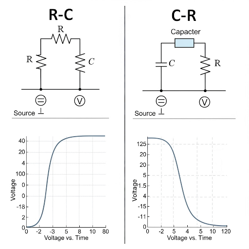
Exactly! This is known as a low-pass filter. At zero frequency, the circuit's response is unity; however, as frequency increases, the impedance of the capacitor decreases.

How do we express that behavior mathematically?
Good question! The transfer function can be represented as V(s) = 1/(1+sRC). Remember this format: it helps us understand various circuit behaviors.
Understanding C-R Circuits
🔒 Unlock Audio Lesson
Sign up and enroll to listen to this audio lesson

Now, let's discuss C-R circuits. How do these differ from R-C circuits in terms of frequency response?

I think C-R circuits let high frequencies pass, right?
Correct! This high-pass filter characteristic allows signals above the corner frequency to pass while attenuating lower ones. Can anyone tell me about the transfer function of the C-R circuit?

Is it something like 1/(sRC + 1)?
Yes, precisely! Just like R-C circuits, it's the poles and zeros that define their behavior, significantly affecting the corner frequency.
Analyzing Frequency Response
🔒 Unlock Audio Lesson
Sign up and enroll to listen to this audio lesson
Now, how do we visualize the frequency response? Bode plots are useful for this. Can anyone explain why we transform the frequency scale?
To more easily see the changes in gain over a range of frequencies?
Exactly! This is why we can represent it on a logarithmic scale, showing linear behavior in decibels. What happens at the corner frequency?
The gain rolls off, typically at -3 dB!
Right! Keep in mind the slope beyond the corner frequency reflects the pole's influence, which introduces a -20 dB/decade roll-off. Remember these key points!
Poles and Corner Frequencies
🔒 Unlock Audio Lesson
Sign up and enroll to listen to this audio lesson
Let's consider the poles of our transfer functions again. How do these relate to the cutoff frequency?
The pole location directly determines where the cutoff frequency lies, right?
Absolutely! The cutoff frequency can be derived from the pole’s Laplace domain representation. Keep that relationship in mind when designing circuits!
Does this mean that in cascaded circuits we must consider the interaction of different poles?
Precisely! When we cascade R-C and C-R circuits, their respective poles must be analyzed to ensure the desired frequency response is achieved.
Practical Implications of R-C and C-R Circuits
🔒 Unlock Audio Lesson
Sign up and enroll to listen to this audio lesson
Finally, let's discuss the practical implications. When would we use an R-C circuit vs. a C-R circuit?
R-C circuits are great for signal conditioning in low frequencies, like audio systems?
Exactly! Meanwhile, C-R circuits are better for removing noise in signals, like high-frequency communication systems.
So, understanding both types is crucial for effective circuit design?
Yes, it's all about matching the circuit response to your specific application needs. Great discussions today!
Introduction & Overview
Read summaries of the section's main ideas at different levels of detail.
Quick Overview
Standard
The section focuses on the analysis of R-C and C-R circuits in the Laplace domain, highlighting their transfer functions, behavior at different frequency ranges, and resulting Bode plots. Key characteristics, such as pass band and stop band behavior, are explored along with the significance of corner frequencies and poles.
Detailed
Detailed Summary
In this section, we analyze the frequency responses of R-C and C-R circuits by transforming the circuits into the Laplace domain. We begin by defining the input and output voltages in terms of the Laplace variable s, establishing transfer functions for both circuits. The comparison reveals that, in the R-C circuit, the transfer function shows a low-pass filter characteristic, allowing low frequencies to pass through while attenuating high frequencies. Conversely, the C-R circuit exhibits a high-pass filter behavior, where low frequencies are blocked, and higher frequencies are allowed to pass.
The discussion includes transformation of frequency response to the Fourier domain, where we can derive gain and phase plots. Specific frequency points of interest are identified, such as the corner frequency where the circuit begins to roll off. The phase shifts at various frequency ranges provide a deeper understanding of the circuit dynamics. Notably, both circuits display essential behaviors such as gaining a certain constant level in the mid-frequency range and exhibiting a roll-off of -20 dB/decade beyond the corner frequencies.
The significance of the pole location within the Laplace transfer function is elucidated, establishing a direct relationship between the pole and the corner frequency. This leads to practical implications, such as the cascading of these circuits while accounting for the loading effects that may alter the overall frequency response.
Youtube Videos

Audio Book
Dive deep into the subject with an immersive audiobook experience.
Circuit Analysis in Laplace Domain
Chapter 1 of 5
🔒 Unlock Audio Chapter
Sign up and enroll to access the full audio experience
Chapter Content
So, similar to the C-R circuit again here what you are doing is that we are taking the circuit into Laplace domain, namely the impedance of both the elements we are going in Laplace domain for C it is and this is directly same as this R. And then input it is V_in in Laplace domain s and then the corresponding output also we are considering in Laplace domain which is V(s).
Detailed Explanation
In this chunk, we begin by analyzing the circuits in the Laplace domain, which is a mathematical approach that allows us to handle differential equations easily. In the Laplace domain, we express the circuit components like resistors (R) and capacitors (C) in terms of their impedances. For example, the impedance of a capacitor is represented differently than that of a resistor, which helps us analyze the circuit more effectively. By transforming the circuit from the time domain to the Laplace domain, we can focus on how the circuit behaves in response to various inputs.
Examples & Analogies
Think of it like translating a book from one language to another. Just as each word might change, the underlying meaning remains intact. Here, we are changing how we represent the components of the circuits to make our calculations easier.
Frequency Response Analysis
Chapter 2 of 5
🔒 Unlock Audio Chapter
Sign up and enroll to access the full audio experience
Chapter Content
Now, to get the frequency response as I said for the previous case what you have to do, we have to take this replace this s by jω or rather I was having say sigma part in s which I am making it 0.
Detailed Explanation
To analyze the frequency response, we replace 's' in our equations with 'jω', where 'j' is the imaginary unit and 'ω' is the angular frequency. This transformation allows us to analyze how the circuit responds at different frequencies. By making the real part of 's' (σ) equal to zero, we isolate the frequency component, thus examining only how the 'imaginary' parts interact. This step is crucial in understanding the output behavior of the circuit as frequency changes.
Examples & Analogies
Imagine tuning a radio to different stations. Replacing 's' with 'jω' is like finding which frequency gives you the clearest reception. You're fine-tuning your machine to hear what the circuit will output at designated frequencies.
Plotting Magnitude and Phase
Chapter 3 of 5
🔒 Unlock Audio Chapter
Sign up and enroll to access the full audio experience
Chapter Content
Again here what you can do? We can plot the magnitude. So, if we consider the | | and with respect to ω. So, if you see here at low frequency; if we ignore this part with respect to 1, then the corresponding magnitude it is 1.
Detailed Explanation
In this part, we are discussing how to plot the circuit's magnitude response against frequency (ω). At lower frequencies, we note that the magnitude is close to 1, meaning the output signal closely resembles the input signal. As the frequency increases, the behavior changes significantly, and we must analyze how the components interact over the frequency spectrum. This is visualized in a magnitude plot, allowing us to see where the input and output behave similarly and where they diverge.
Examples & Analogies
Consider a dimmer switch in your home. At low settings (low frequency), the light is bright (output signal is strong). As you dim it more (increase frequency), the light gradually dims (output signal weakens), allowing us to see how the circuit illuminates at various settings.
Gain and Attenuation
Chapter 4 of 5
🔒 Unlock Audio Chapter
Sign up and enroll to access the full audio experience
Chapter Content
But then if you go to higher and higher frequency and if this part it is dominating over this 1, then the magnitude wise what we will be seeing here it is 1 by ω nature.
Detailed Explanation
As frequency increases, the output's magnitude response begins to behave as '1/ω', indicating that the signal is being attenuated. This characteristic behavior is typical of low-pass filters, where lower frequencies are allowed to pass through, while higher frequencies are diminished or blocked. This transition showcases the filtering effect of the circuit, crucial in many signal processing applications.
Examples & Analogies
Think of it like a sponge soaking up water. At first, it absorbs comfortably (low frequencies passing through). As you pour in more water (higher frequencies), it starts overflowing (signal weakening). The sponge's ability to handle the water represents the circuit's ability to manage frequency changes.
Behavior Beyond Corner Frequency
Chapter 5 of 5
🔒 Unlock Audio Chapter
Sign up and enroll to access the full audio experience
Chapter Content
So, I should say if I call this is ω where ω RC = 1 which means ω = 1/RC.
Detailed Explanation
The 'corner frequency' (or cutoff frequency) is significant as it marks a transition point in circuit behavior. At this frequency, the effects of resistance (R) and capacitance (C) balance out, leading to a shift from passing to attenuating signals. Understanding this point is crucial in designing circuits to meet specific frequency requirements, especially in filters and amplifiers.
Examples & Analogies
Imagine a rollercoaster. As you ascend (lower frequencies), you build momentum. At the peak (corner frequency), you're at the highest point, transitioning to a thrilling drop (higher frequencies). Knowing this peak height helps engineers design safe rides, just like understanding corner frequency aids in effective circuit design.
Key Concepts
-
R-C Circuit: A low-pass filter that allows low frequencies to pass.
-
C-R Circuit: A high-pass filter that allows high frequencies to pass.
-
Transfer Function: Represents input-output relationships in the Laplace domain.
-
Corner Frequency: The point at which gain begins to roll off.
-
Bode Plot: A graphical method to represent frequency response.
Examples & Applications
An R-C circuit used in audio equipment to filter low-frequency noise.
A C-R circuit implemented in radio receivers to eliminate low-frequency noise.
Memory Aids
Interactive tools to help you remember key concepts
Rhymes
For an R-C, let low frequencies play, while in C-R, the highs lead the way.
Stories
Once, in a land of signals and waves, there lived an R-C circuit that loved low frequencies. But nearby, a C-R circuit resided, always favoring the high tones, proving opposites attract in the signal town.
Memory Tools
LFS for R-C (Low Frequencies Supported) and HFS for C-R (High Frequencies Supported).
Acronyms
LPF for R-C (Low Pass Filter) and HPF for C-R (High Pass Filter).
Flash Cards
Glossary
- RC Circuit
A circuit composed of a resistor (R) and a capacitor (C) that exhibits low-pass filter characteristics.
- CR Circuit
A circuit consisting of a capacitor (C) followed by a resistor (R) that behaves like a high-pass filter.
- Transfer Function
A mathematical representation of the relationship between the input and output of a system in the Laplace domain.
- Corner Frequency
The frequency at which the gain of a circuit begins to roll off, typically -3 dB in magnitude.
- Bode Plot
A graphical representation of the frequency response of a system, displaying gain and phase across a range of frequencies.
Reference links
Supplementary resources to enhance your learning experience.