
Magnitude and Phase Plot Analysis
Enroll to start learning
You’ve not yet enrolled in this course. Please enroll for free to listen to audio lessons, classroom podcasts and take practice test.
Interactive Audio Lesson
Listen to a student-teacher conversation explaining the topic in a relatable way.
Introduction to Frequency Response
🔒 Unlock Audio Lesson
Sign up and enroll to listen to this audio lesson

Today, we will delve into the concept of frequency response in RC circuits. Can anyone explain what frequency response refers to?

Frequency response shows how the output signal of a circuit varies with the input frequency, right?
Excellent! That's correct. We analyze the magnitude and phase of the output compared to the input. What do you think happens at low frequencies?

The circuit allows signals to pass through without much change?
Exactly, at low frequencies, the gain remains constant, close to one. This is a characteristic of a low-pass filter.

What about at high frequencies?
Good question! At higher frequencies, the gain decreases, typically at a rate of -20 dB per decade. This is often due to the increased capacitive reactance.

I still find it tricky to visualize that change in gain!
Let's visualize this with a graph later. Remember, understanding how frequency affects gain is crucial in designing circuits.
Understanding Magnitude and Phase
🔒 Unlock Audio Lesson
Sign up and enroll to listen to this audio lesson

Now, let's discuss how to create and interpret magnitude and phase plots. How do you think we can represent these parameters?
By using graphs, maybe plotting gain against frequency?
Exactly! Magnitude and phase plots are typically shown on logarithmic scales. This helps us to analyze behaviors across a wide range of frequencies.
What's the significance of the corner frequency?
Great question! The corner frequency marks the transition point where the circuit’s behavior shifts from passing to attenuating signals drastically.
How does that relate to the poles of the transfer function?
Fantastic inquiry! The location of poles in the transfer function directly influences the corner frequency. We can establish a relationship based on the transfer function’s properties.
Bode Plot Insights
🔒 Unlock Audio Lesson
Sign up and enroll to listen to this audio lesson
Let's now focus on Bode plots. What do you all understand by a Bode plot?
I think it's a way to visualize the frequency response on logarithmic scales.
Exactly! Bode plots allow us to easily interpret magnitude and phase shifts within circuits. Can anyone recall the slope behavior?
At the corner frequency, the slope drops to -20 dB per decade!
Spot on! This consistent slope makes it easier to predict circuit behavior without calculating each frequency individually. Great job, everyone!
Recap and Applications
🔒 Unlock Audio Lesson
Sign up and enroll to listen to this audio lesson
To wrap up, can anyone summarize the key concepts we've learned about magnitude and phase plot analysis?
RC circuits allow signals to pass easily at low frequencies but attenuate at high frequencies.
The corner frequency is vital as it shows the transition from pass to stop band.
Bode plots help visualize these behaviors clearly.
Excellent summary! Remember, understanding these concepts is crucial for designing effective circuits, especially amplifiers.
Introduction & Overview
Read summaries of the section's main ideas at different levels of detail.
Quick Overview
Standard
In this section, we explore the frequency response of RC circuits by analyzing the magnitude and phase plots. Key concepts such as the corner frequency, gain behavior in low and high frequencies, and the characteristics of Bode plots are highlighted, showing how the poles of the transfer function determine these responses.
Detailed
Detailed Summary
The frequency response of RC circuits is crucial for understanding how these components behave across different frequencies. In this section, we start by transforming the circuit to the Laplace domain to develop the transfer function. By substituting the Laplace variable s with jω, we obtain the frequency response in the Fourier domain.
The analysis reveals two main behaviors:
1. At low frequencies, the circuit acts as a low pass filter, allowing signals to pass through without significant attenuation, demonstrated by constant gain of approximately 1.
2. As frequency increases beyond a certain point called the corner frequency (ω=1/RC), the gain rolls off at -20 dB per decade due to the predominance of the capacitive reactance.
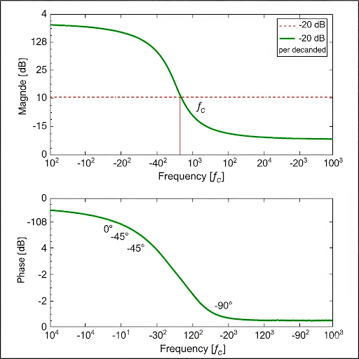
Additionally, phase shifts are examined, with a 0° phase shift at low frequencies transitioning to -90° at high frequencies, reflecting the nature of capacitive behavior. The importance of Bode plots, which represent these responses on logarithmic scales, is discussed, emphasizing that the relationship between the poles of the transfer function and the cutoff frequency can be easily deduced. Understanding these concepts is fundamental in electronic circuit design, particularly in amplifying signals effectively.
Youtube Videos

Audio Book
Dive deep into the subject with an immersive audiobook experience.
Introduction to Frequency Response
Chapter 1 of 5
🔒 Unlock Audio Chapter
Sign up and enroll to access the full audio experience
Chapter Content
To get the frequency response as I said for the previous case what you have to do, we have to take this replace this s by jω or rather I was having say sigma part in s which I am making it 0. So, we are dropping this part and that gives us the transfer function in Fourier domain and it becomes.
Detailed Explanation
This chunk introduces how to derive the frequency response from the transfer function. To analyze how the circuit behaves at different frequencies, we replace 's' with 'jω'. This step assumes that sigma, which contributes to damping and stability, is made zero, simplifying our equation to focus solely on the frequency response. The result is the transfer function expressed in the Fourier domain, which is crucial for understanding how the circuit reacts to varying frequencies.
Examples & Analogies
Think of it like tuning a radio: when you tune to different frequencies (like s to jω), you're able to hear different stations. By simplifying our equations this way, we're essentially tuning the circuit to focus on the frequencies of interest.
Magnitude Response
Chapter 2 of 5
🔒 Unlock Audio Chapter
Sign up and enroll to access the full audio experience
Chapter Content
So, again here what you can do? We can plot the magnitude. So, if we consider the | | and with respect to ω. So, if you see here at low frequency; if we ignore this part with respect to 1, then the corresponding magnitude it is 1. But then if you go to higher and higher frequency and if this part it is dominating over this 1, then the magnitude wise what we will be seeing here it is 1 by ω nature.
Detailed Explanation
In this chunk, we plot the magnitude of the transfer function against frequency (ω). At low frequencies, the magnitude remains constant (1), indicating that the circuit allows these frequencies to pass through. However, as frequency increases beyond a certain point, the circuit starts to behave like a filter, and the output magnitude decreases; mathematically, it becomes proportional to 1/ω. This indicates the circuit's transition from passband to stopband behavior.
Examples & Analogies
Imagine a water pipe: at low flow rates (low frequencies), water flows freely. But as you try to push water through at higher rates (higher frequencies), the pipe constricts (the capacitor presents more impedance), and less water gets through, representing the decrease in output signal.
Phase Response
Chapter 3 of 5
🔒 Unlock Audio Chapter
Sign up and enroll to access the full audio experience
Chapter Content
Now, the similar to the previous case here again we can make the phase plot and then the if you consider the phase plot at very low frequency this part it is almost 0. So, we do have 0 phase shift. So, you can see that the phase shift here it is 0°. So, this y-axis is the phase shift offered by this network.
Detailed Explanation
This section covers the phase response of the circuit. Initially, at low frequencies, the phase shift is 0°, meaning the output signal is in sync with the input signal. As frequency increases, the circuit introduces a phase shift. By plotting this phase behavior against frequency, we gain insights into how the circuit alters the timing of the output signal relative to the input, which is critical in applications involving signal processing.
Examples & Analogies
Think of a dance party where everyone is moving in sync (0° phase shift) at the beginning. As the music tempo speeds up, some dancers fall out of sync (introducing a phase shift) - similarly, the circuit’s behavior changes from being perfectly in time to introducing delays in signal transmission.
Bode Plot Representation
Chapter 4 of 5
🔒 Unlock Audio Chapter
Sign up and enroll to access the full audio experience
Chapter Content
So, we need to change this scale into logarithmic form and magnitude also we like to change in logarithmic form.
Detailed Explanation
In this part, the discussion transitions to using Bode plots, which represent frequency response in a logarithmic scale for both frequency and magnitude. This approach helps visualize the data better, especially for circuits that cover a wide frequency range. By changing to logarithmic scales, we can easily observe trends like corner frequencies and gain roll-off, enabling engineers to analyze performance at different frequencies more effectively.
Examples & Analogies
Think of reading a map. When you zoom in (logarithmic scale), details become clearer at specific areas, allowing you to track your route better. The Bode plot does the same for frequency response, helping identify important characteristics of the circuit's behavior.
Corner Frequency and Roll-off
Chapter 5 of 5
🔒 Unlock Audio Chapter
Sign up and enroll to access the full audio experience
Chapter Content
So, we can say that this corner frequency whether it is in; so, this is gain in gain or magnitude in dB. So, these this corner frequency and whether it is in this frequency response or in Bode plot, it is related to this location of the pole.
Detailed Explanation
This chunk elaborates on the importance of the corner frequency in frequency response plots. The corner frequency marks the point where the gain begins to roll off, typically around -3 dB in a Bode plot. Understanding the relationship between the pole's location in the transfer function and the corner frequency is essential, as it allows engineers to predict the behavior of the circuit. The pole’s influence over the corner frequency is critical when designing filters or amplifiers based on desired performance.
Examples & Analogies
Imagine a sports car’s handling. The corner (cutoff frequency) is where the car starts losing grip (gain drops) due to higher speeds. At that corner speed, understanding how much grip you have left is crucial to avoid spinning out, just like knowing the corner frequency helps maintain circuit performance.
Key Concepts
-
Frequency Response: Represents how output varies with input frequency.
-
Magnitude and Phase Plots: Graphical representation of gain and phase shift.
-
Corner Frequency: The transition frequency where gain begins to attenuate.
-
Bode Plot: A tool that simplifies analyzing amplitude and phase shifts.
Examples & Applications
In an RC circuit, at low frequencies (below corner frequency), the voltage gain might be 1, indicating no attenuation of the signal.
In a Bode plot of an RC circuit, the magnitude plot will typically show a decrease of -20 dB per decade past the corner frequency.
Memory Aids
Interactive tools to help you remember key concepts
Rhymes
At low frequency, the signal's fate, is to pass right through, not hesitate.
Stories
Imagine a bouncer named RC at a club, low frequencies get in without a thud, but as the beat drops, high frequencies fade out, he sends them away with no doubt.
Memory Tools
To remember the frequency response: 'Low In, High Out, Corner Count!' - emphasizes the order of operations.
Acronyms
F.R.E.C
Frequency Response
Gain
Roll-off
Corner frequency - key ideas of frequency analysis.
Flash Cards
Glossary
- Frequency Response
The analysis of how the output signal of a circuit responds to varying frequencies of the input signal.
- Magnitude Plot
A graphical representation showing the gain of an electrical circuit as a function of frequency.
- Phase Plot
A graphical representation indicating the phase shift of the output signal relative to the input signal at various frequencies.
- Corner Frequency
The frequency at which the gain of the circuit begins to significantly drop, usually marked by a -3 dB point.
- Bode Plot
A logarithmic plot representing the magnitude and phase of a system's frequency response.
Reference links
Supplementary resources to enhance your learning experience.