
Frequency Response of CE and CS Amplifiers (Part B)
Enroll to start learning
You’ve not yet enrolled in this course. Please enroll for free to listen to audio lessons, classroom podcasts and take practice test.
Interactive Audio Lesson
Listen to a student-teacher conversation explaining the topic in a relatable way.
Introduction to Frequency Response
🔒 Unlock Audio Lesson
Sign up and enroll to listen to this audio lesson

Welcome to today's lesson on frequency response! Can anyone tell me what frequency response means in the context of amplifiers?

Isn’t it how the output signal changes with varying input frequencies?
Exactly! Frequency response describes how the output amplitude and phase shift relative to the input changes as we vary the input frequency. We often use transfer functions to explore this.

What do you mean by transfer functions?
Great question! A transfer function is a mathematical representation of the output-input relationship in the Laplace domain. For a simple RC circuit, it helps us understand how the circuit behaves at different frequencies.

Can you show us how that’s done?
Certainly! We derive the transfer function by taking the Laplace transform of the circuit equations, yielding a function like V(s) = ... .

But how does substituting 's' with 'jω' work?
When calculating frequency response, we replace 's' with 'jω', which gives us the function in the frequency domain. This addresses how the output signal behaves specifically at certain frequencies.
In summary, we learned that the transfer function is crucial in analyzing how amplifiers respond to different frequencies.
Magnitude and Phase Response
🔒 Unlock Audio Lesson
Sign up and enroll to listen to this audio lesson

Now, let’s talk about magnitude and phase response. What happens to the magnitude of the output signal as frequency increases?
It starts at 1 and then goes down, right?
Exactly! At low frequencies, the output is close to the input, but as frequency increases, it behaves as 1/ω. This creates a hyperbolic curve.
And what about the phase shift?
Good point! The phase starts at 0° and gradually moves to -90° as we approach high frequencies, indicating how the output lags behind the input. Can anyone see the relationship between magnitude and phase?
I think the higher attenuation correlates with more phase shift, doesn’t it?
Spot on! The phase shift increases with frequency, reflecting the attenuation experienced by the circuit. Let’s summarize: the magnitude reduces as 1/ω, and the phase shifts from 0° to -90°.
Understanding Bode Plots
🔒 Unlock Audio Lesson
Sign up and enroll to listen to this audio lesson
Now, I'd like to touch on Bode plots. What do we use Bode plots for?
They show how gain and phase shift vary over a wide frequency range.
Exactly! We use logarithmic scales for frequency and gain to better visualize the response. This helps in identifying corner frequencies where the response changes.
Is the corner frequency related to the pole?
Yes! The pole of the transfer function determines the corner frequency. As the pole moves, so does the corner frequency. Remember this: 'Pole determines the roll-off.'
So poles directly affect our amplifier's performance?
Absolutely! Understanding poles helps us design better amplifiers. To summarize, Bode plots provide essential visual insights into amplifier performance and corner frequencies can be traced back to pole positions.
Cascading Circuits
🔒 Unlock Audio Lesson
Sign up and enroll to listen to this audio lesson
Let's now explore cascading RC and CR circuits. Why might we cascade circuits?
To produce a specific frequency response that's not achievable with a single circuit?
Exactly! Cascading allows us to design complex responses. But what challenges might arise from cascading?
Loading effects could mess with the response, right?
Indeed! To mitigate loading effects, we use ideal voltage amplifiers in between. Can anyone explain how this helps?
It ensures that the output of one stage doesn't load the next stage?
Precisely! To sum up, cascading enhances circuit functionality but requires careful management of loading effects for optimal performance.
Summary and Review
🔒 Unlock Audio Lesson
Sign up and enroll to listen to this audio lesson
As we conclude, can anyone summarize what we've learned about frequency response?
We learned about transfer functions, how magnitude and phase responses behave, Bode plots, and the implications of cascading circuits.
It’s also clear how poles impact the corner frequency and overall performance.
Excellent recap! Remember, the analysis of frequency response is crucial for designing effective amplifiers in analog electronics. Keep exploring these concepts!
Introduction & Overview
Read summaries of the section's main ideas at different levels of detail.
Quick Overview
Standard
The section covers the frequency response of RC circuits used in CE and CS amplifiers, explaining concepts such as transfer functions, magnitude and phase plots, corner frequencies, and their significance in amplifier design.
Detailed
Frequency Response of CE and CS Amplifiers (Part B)
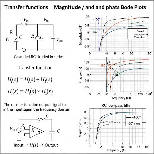
This section focuses on the frequency response of common emitter (CE) and common source (CS) amplifiers, utilizing RC circuits. It commences with an analysis of the RC circuit in the Laplace domain, establishing a direct relationship between the circuit's impedance and its behavior in frequency response.
Key points include:
-
Transfer Functions: The output voltage in the Laplace domain is derived, resulting in a transfer function. By substituting
swithjω, the function is then evaluated for frequency response. - Magnitude and Phase Plots: The magnitude response is observed initially as a flat curve at low frequencies (equal to 1), transitioning to a hyperbolic behavior (1/ω) at higher frequencies, indicating attenuation. The phase response begins at 0° and approaches -90° as frequency increases.
- Bode Plots: The transition from linear to logarithmic scales emphasizes corner frequencies. The relationship between poles and corner frequencies is clarified, helping identify how the location of poles affects the cutoff frequency.
- Cascading Circuits: The interplay between RC and CR circuits is examined, showcasing how cascading these components can lead to complex frequency responses defined by their individual poles and zeros. The loading effect and its mitigation are also covered.
Through these discussions, the section provides detailed insights into the frequency behavior of amplifiers, critical for their effective design and application in analog electronics.
Youtube Videos

Audio Book
Dive deep into the subject with an immersive audiobook experience.
Introduction to Frequency Response in R-C Circuits
Chapter 1 of 5
🔒 Unlock Audio Chapter
Sign up and enroll to access the full audio experience
Chapter Content
So, welcome back to this R-C circuit frequency response after the short break. Similar to the C-R circuit again here what you are doing is that we are taking the circuit into Laplace domain...
Detailed Explanation
In this chunk, we introduce the concept of frequency response in R-C circuits. The frequency response describes how the output of a circuit varies with different input frequencies. The approach begins by transforming the circuit into the Laplace domain, which allows for easier analysis using its impedance. The input voltage (V_in) and output voltage (V_o) are expressed in the Laplace domain (with 's' representing the complex frequency). By analyzing the circuit, we derive a transfer function that will help us understand how signals of various frequencies are affected by the circuit.
Examples & Analogies
Think of the Laplace domain as a translator for frequencies. Just as a translator helps communicate between speakers of different languages, the Laplace transform allows us to analyze circuits in a way that makes it easier to understand how they react to different frequencies.
Understanding Transfer Functions
Chapter 2 of 5
🔒 Unlock Audio Chapter
Sign up and enroll to access the full audio experience
Chapter Content
Now, to get the frequency response... we have to take this replace this s by jω...
Detailed Explanation
This chunk focuses on obtaining the frequency response from the transfer function. By substituting 's' with 'jω' (where j represents the imaginary unit), we convert our analysis from the Laplace domain to the Fourier domain. This gives us the amplitude and phase responses of the circuit, which are essential for understanding how the circuit behaves at different frequencies.
Examples & Analogies
Imagine tuning a radio to different stations (frequencies). Each station has a unique signal, much like how each frequency in our circuit's analysis generates a different response. When we tune the radio, we’re essentially replacing 's' with 'jω' to find the strength and clarity (amplitude and phase) of the desired station.
Magnitude and Phase Plots
Chapter 3 of 5
🔒 Unlock Audio Chapter
Sign up and enroll to access the full audio experience
Chapter Content
So, again here what you can do? We can plot the magnitude...
Detailed Explanation
In this section, we learn how to plot the frequency response in terms of magnitude and phase. The magnitude indicates how much of the input signal is passed through at various frequencies. Early on, at low frequencies, the output closely resembles the input (magnitude of 1). However, as the frequency increases, the circuit behaves differently, leading to a decay in magnitude, particularly beyond a certain frequency (the cutoff frequency, ω_c). The phase plot illustrates the phase shift incurred by the circuit at different frequencies. Initially, there’s no phase shift (0°), but it becomes negative as frequency increases, indicating a lag in the output signal compared to the input signal.
Examples & Analogies
This is akin to a musical instrument. At low notes (low frequencies), the sound comes out clearly, but as you play higher notes (higher frequencies), the sound may become distorted (the output changes). Similarly, the phase plot shows how the timing of the sound from the instrument shifts as notes change.
Bode Plots and Corner Frequency
Chapter 4 of 5
🔒 Unlock Audio Chapter
Sign up and enroll to access the full audio experience
Chapter Content
Now, similar to the previous case again since we like to see the wide range of frequency...
Detailed Explanation
Bode plots are a graphical method used to represent the frequency response of systems. They allow engineers to visualize how gain (amplitude) and phase vary with frequency on a logarithmic scale. The corner frequency is the frequency point at which the magnitude falls to −3 dB, indicating where the circuit transitions from passing signal effectively to beginning to attenuate it. Understanding the corner frequency gives insights into the practical operating range of the circuit.
Examples & Analogies
Think of a ride at an amusement park that accelerates up to a certain speed (gaining excitement) but starts to slow down after reaching a peak speed. The corner frequency in our circuit is like that peak speed. Below it, the ride is thrilling, but after it, the excitement diminishes, just as signals do in our circuit beyond the corner frequency.
Role of Poles in Frequency Response
Chapter 5 of 5
🔒 Unlock Audio Chapter
Sign up and enroll to access the full audio experience
Chapter Content
Yeah, this part we already have covered; Bode plot we already have covered yeah...
Detailed Explanation
In this chunk, we explore the significance of poles in determining frequency response. The location of a pole in the transfer function impacts the magnitude and phase characteristics at various frequencies. It plays a critical role in determining the behavior of the circuit, especially in shaping the corner frequency. A pole signifies a point where the output starts becoming limited or 'cut-off', impacting how signals at certain frequencies are handled by the circuit.
Examples & Analogies
Imagine a traffic control system where certain intersections (poles) restrict the flow of cars (signals). Just as these intersections can cause delays or smooth transitions in traffic, the poles in our circuit control how signals of different frequencies are processed – shaping the output we eventually see.
Key Concepts
-
Frequency Response: The behavior of a circuit output relative to input frequency.
-
Magnitude Response: Reflects how the output amplitude varies with frequency.
-
Phase Response: Indicates the phase shift between input and output signals as frequency changes.
-
Bode Plot: A graphical representation of magnitude and phase responses as functions of logarithmic frequency.
-
Poles and Zeros: Critical points in the transfer function that impact circuit behavior.
Examples & Applications
Example of a simple RC circuit showing the frequency response transition from low to high frequencies and how the output magnitude decreases.
Example of Bode plot illustrating a transfer function for a common emitter amplifier and its significant corner frequency.
Memory Aids
Interactive tools to help you remember key concepts
Rhymes
When frequency does climb higher, gain will drop, like a tired flyer.
Stories
Imagine an amplifier like a music band. As the tempo increases fast, the singer struggles to keep the pitch right, representing how gain decreases with higher frequency.
Memory Tools
P.U.B.K. — Poles and zeros are Unified in Bode representation of the frequency response.
Acronyms
F.R.A.M.E. — Frequency Response, Amplitude, Magnitude, and Edge (corner frequency).
Flash Cards
Glossary
- Transfer Function
A mathematical representation that defines the relationship between input and output of a system in the Laplace domain.
- Bode Plot
A graph representing the gain and phase shift of a system, plotted against logarithmic frequency.
- Corner Frequency
The frequency at which the response of a system deviates from its flat or dominant behavior, typically defined where the gain is -3 dB.
- Pole
A value in the Laplace domain that determines the stability and frequency response characteristics of a circuit.
- Loading Effect
The impact on the output of a circuit when connected to another circuit, which may affect the network's performance.
Reference links
Supplementary resources to enhance your learning experience.