
MOTION IN A PLANE WITH CONSTANT ACCELERATION
Enroll to start learning
You’ve not yet enrolled in this course. Please enroll for free to listen to audio lessons, classroom podcasts and take practice test.
Interactive Audio Lesson
Listen to a student-teacher conversation explaining the topic in a relatable way.
Understanding Constants in Motion
🔒 Unlock Audio Lesson
Sign up and enroll to listen to this audio lesson

Today, we're going to discuss motion in a plane with constant acceleration. First, who can explain what constant acceleration means?

It means the acceleration doesn't change over time.
Exactly! So if we know the initial velocity, we can find the velocity after some time. Can anyone remind us of the formula?

Isn't it v = v0 + at?
Correct! This formula will help us determine how fast the object is moving after a given time. Now, let's move on to thinking about motion in two dimensions.

How would that look? Does it still use the same equations?
Great question! Yes, we adapt the equations to the x and y components. Remember, the motion can be analyzed separately along each axis. To summarize, we use the equations we discussed, but split them for each dimension.
Position Change over Time
🔒 Unlock Audio Lesson
Sign up and enroll to listen to this audio lesson

Now, let’s dive into position changes. How do we represent the position of an object when it's accelerating?

Isn't the formula r = r0 + v0t + (1/2)at²?
Absolutely! This equation gives us the new position based on the initial position and changes due to velocity and acceleration. Can someone break this down for the x and y components?
Sure! For the x direction, it's x = x0 + v0x t + (1/2) ax t², and for y, it's y = y0 + v0y t + (1/2) ay t².
Well done! Knowing how to separate these components is key when dealing with two-dimensional motion.
Connecting Velocity and Position
🔒 Unlock Audio Lesson
Sign up and enroll to listen to this audio lesson
Let's talk about how position changes can be related to velocity. Why do you think it matters to consider both?
Because knowing the velocity at the start helps us predict where the object will be later!
Exactly! The velocity gives us insight into how the position updates over time. Can you derive the position formula based on the velocity?
We can integrate velocity over time! If we take v = dx/dt, then integrating gives us the position.
Wonderful application of calculus! Always remember the relationship between these concepts.
Applications of Motion Equations
🔒 Unlock Audio Lesson
Sign up and enroll to listen to this audio lesson
Now that we understand the equations for motion, how can we apply them to problem-solving?
We could find out how far an object has traveled after a specific time with a known acceleration.
Correct! Always start with what you know from the problem and plug those values into the right formulas. What about finding the final velocity after a set distance?
We could use the equation involving displacement and initial velocity!
Exactly! Practice will reinforce these concepts, so let’s tackle some exercises to solidify our understanding.
Introduction & Overview
Read summaries of the section's main ideas at different levels of detail.
Quick Overview
Standard
In this section, we explore the dynamics of objects moving in a plane with constant acceleration. Key equations governing acceleration, velocity, and displacement are presented, illustrating how these properties interact over time. The section emphasizes the importance of component analysis for understanding motion in multiple dimensions.
Detailed
Motion in a Plane with Constant Acceleration
In this section, we examine the motion of a particle moving in the x-y plane with a constant acceleration. The primary focus is on how the velocity and position of the object change over time due to this steady acceleration.
Key Relationships:
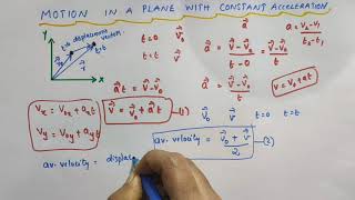
- Velocity: The change in velocity (v) from an initial velocity (v0) after a time interval (t) can be expressed as:
- \[ v = v_0 + a t \]
where \( a \) is the constant acceleration, affecting both x and y components of velocity as: - \[ v_x = v_{0x} + a_x t \]
- \[ v_y = v_{0y} + a_y t \]
- Position: The position vector change over time is given by:
- \[ r = r_0 + v_0 t + \frac{1}{2} a t^2 \]
where \( r_0 \) is the initial position. This leads to component-wise representation of position: - \[ x = x_0 + v_{0x} t + \frac{1}{2} a_x t^2 \]
- \[ y = y_0 + v_{0y} t + \frac{1}{2} a_y t^2 \]
The analysis demonstrates that motion in a plane can be treated as two independent one-dimensional motions along perpendicular axes. Understanding these relationships is crucial for tackling complex two-dimensional motion problems effectively.
Youtube Videos

Audio Book
Dive deep into the subject with an immersive audiobook experience.
Concept of Constant Acceleration
Chapter 1 of 4
🔒 Unlock Audio Chapter
Sign up and enroll to access the full audio experience
Chapter Content
Suppose that an object is moving in x-y plane and its acceleration a is constant. Over an interval of time, the average acceleration will equal this constant value.
Detailed Explanation
When an object is moving with constant acceleration in a plane, it means that the rate at which its velocity is changing remains consistent over time. The acceleration does not fluctuate, resulting in uniform changes to the object's speed and direction during its motion.
Examples & Analogies
Imagine a car entering a highway and speeding up steadily. If the car increases its speed at a constant rate of 10 km/h every second, that is constant acceleration. No matter how fast the car is going, as long as it accelerates by the same amount each second, it demonstrates constant acceleration.
Velocity Change Equation
Chapter 2 of 4
🔒 Unlock Audio Chapter
Sign up and enroll to access the full audio experience
Chapter Content
Let the velocity of the object be v0 at time t = 0 and v at time t. Then, by definition av = (v - v0) / t, or v = v0 + at.
Detailed Explanation
The equation v = v0 + at expresses the relationship between the final velocity (v), initial velocity (v0), the acceleration (a), and the time taken (t). It shows how the velocity of an object changes from its initial state due to constant acceleration. 'a' is multiplied by 't' to find how much velocity has changed from v0 to v.
Examples & Analogies
Consider a skateboarder starting from rest at the top of a hill (v0 = 0). If the skateboard accelerates downward at 2 m/s², after 3 seconds, their velocity will be 0 m/s + (2 m/s² * 3 s) = 6 m/s at the bottom. This formula is the key to understanding how quickly they reach that speed.
Position Change Equation
Chapter 3 of 4
🔒 Unlock Audio Chapter
Sign up and enroll to access the full audio experience
Chapter Content
Let ro and r be the position vectors of the particle at time 0 and t. The displacement is given by: r = ro + vt + (1/2) at².
Detailed Explanation
This equation shows how the position of an object changes over time under constant acceleration. The first part, ro, represents the initial position, while the term (1/2)at² accounts for the distance covered due to acceleration. By adding these two components together with vt (the distance traveled due to the velocity), you get the total distance from the starting point.
Examples & Analogies
Imagine you throw a ball straight up into the air. Initially, it's at your hand's height (ro). As it travels upward, its initial velocity moves it further up. However, gravity (the acceleration in this case) will cause it to slow down, change direction, and come back down. The total distance traveled can be calculated with this equation, considering the acceleration due to gravity affects the ball's height.
Breaking Down into Components
Chapter 4 of 4
🔒 Unlock Audio Chapter
Sign up and enroll to access the full audio experience
Chapter Content
In terms of components: x: x = x0 + v0xt + (1/2) ax t² and y: y = y0 + v0yt + (1/2) ay t².
Detailed Explanation
This takes the previous equations and splits them into horizontal (x) and vertical (y) components. Each part shows how to calculate the position based on initial conditions and how much each direction is affected by their respective accelerations. This separation makes it easier to analyze and understand movements in two dimensions.
Examples & Analogies
If you throw a ball, it moves up while also drifting sideways due to wind or your throw angle. By breaking its motion into horizontal and vertical components, you can calculate the ball's path more accurately, ensuring you understand how far it goes in the air and how high it reaches before falling back down.
Key Concepts
-
Velocity changes under constant acceleration, allowing predictions of future motion.
-
Displacement represents the overall change in position, not the path taken.
-
Both position and velocity can be analyzed using component methods in two dimensions.
Examples & Applications
If a car accelerates at 2 m/s² from an initial velocity of 10 m/s, its velocity after 5 seconds will be 20 m/s.
A projectile launched at an angle can be analyzed separately by decomposing its motion into horizontal and vertical components.
Memory Aids
Interactive tools to help you remember key concepts
Rhymes
To find velocity new, just grab the old and add the acceleration too.
Stories
Imagine a car that starts at a stop and speeds up to 60 mph at a steady rate; you can calculate its distance traveled based on its change in speed.
Memory Tools
V = V0 + AT for Velocity, and S = V0T + ½AT^2 for Displacement captures our motion rules.
Acronyms
VDS (Velocity, Displacement, Speed) helps remember the key equations for motion.
Flash Cards
Glossary
- Constant Acceleration
Acceleration that does not change in magnitude or direction over time.
- Velocity
The rate at which an object changes its position, encompassing both speed and direction.
- Displacement
The vector quantity representing the change in position of an object.
- Position Vector
A vector representing the position of a particle in space relative to the origin.
Reference links
Supplementary resources to enhance your learning experience.