
Time History Analysis of MDOF Systems
Enroll to start learning
You’ve not yet enrolled in this course. Please enroll for free to listen to audio lessons, classroom podcasts and take practice test.
Interactive Audio Lesson
Listen to a student-teacher conversation explaining the topic in a relatable way.
Understanding Time History Analysis
🔒 Unlock Audio Lesson
Sign up and enroll to listen to this audio lesson

Today, we will explore time history analysis of MDOF systems. What do you think it involves?

I think it has to do with how structures respond over time.
Exactly! It’s about evaluating the dynamic behavior of structures when subjected to forces, like during an earthquake. Can anyone tell me what we need for this analysis?

We need records of ground acceleration.
Correct! We also need a damping matrix and an accurate time step for calculations. Remember the acronym 'GAD' — Ground acceleration, Damping matrix, and accurate time step.

Why is the time step so critical?
Good question! A proper time step ensures that our analysis captures the dynamics accurately without excessive computation.

What happens if the time step is too large?
If it’s too large, we may miss critical changes in response, leading to inaccurate results. Let's summarize today's talk: Time history analysis is crucial to understanding how structures respond over time under seismic loads.
Numerical Integration Methods in Time History Analysis
🔒 Unlock Audio Lesson
Sign up and enroll to listen to this audio lesson

Now, let's look at the specific numerical integration methods used. Can anyone mention some methods?
Isn't the Newmark-beta method commonly used?
Absolutely! The Newmark-beta method is popular because it balances stability and accuracy well. What other methods do you know?
There’s also the Wilson-θ method and Runge-Kutta methods.
Great! Both Wilson-θ and Runge-Kutta methods are important for ensuring accurate time integration. Let's use the mnemonic 'NRW' for Newmark, Runge, Wilson to remember these methods.
What kinds of structures benefit from these analyses?
Excellent question! Critical infrastructure, like hospitals and bridges, commonly utilizes time history analysis to ensure they can withstand earthquake forces.
Can we summarize what we've learned about integration methods?
Sure! We explored methods like Newmark-beta, Wilson-θ, and Runge-Kutta for analyzing MDOF systems under dynamic loads.
Applications of Time History Analysis
🔒 Unlock Audio Lesson
Sign up and enroll to listen to this audio lesson
Finally, let's discuss the applications of time history analysis. What have you encountered regarding its use?
I heard it’s used for designing buildings that need to be earthquake-resistant.
Correct! It is crucial for designing critical structures. Effective time history analysis verifies that designs will hold up under seismic events.
How does it help with structural modeling?
Excellent point! It checks that the predicted dynamic characteristics match actual performance. This validation is key for engineers.
So, it’s about ensuring the structure will perform safely and effectively?
Exactly! In summary, time history analysis is essential for the design and validation of structures to withstand dynamic loads, especially during earthquakes.
Introduction & Overview
Read summaries of the section's main ideas at different levels of detail.
Quick Overview
Standard
This section covers time history analysis in MDOF systems, detailing the requirements like ground acceleration, damping matrices, and the importance of accurate time steps. It also introduces numerical integration methods that can be employed for the analysis and their applications in designing critical infrastructure.
Detailed
Detailed Summary
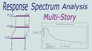
Time history analysis is an essential technique used to examine the complete dynamic behavior of Multiple Degree of Freedom (MDOF) systems when ground motion acceleration records, such as during an earthquake, are available. This analysis involves direct time integration to evaluate the system's response over time, offering insights into how structures respond to seismic loading.
Key Requirements for Time History Analysis:
- Ground Acceleration (
u¨_g(t)): The input data, typically obtained from accelerometer records, which represents the acceleration of the ground during seismic events. - Damping Matrix: A representation of energy dissipation in the system, critical for accurately capturing dynamic responses.
- Accurate Time Step: A well-chosen time step is vital; too large can lead to errors, while too small increases computational demand.
Numerical Integration Methods:
Key numerical techniques used for time history analysis include:
- Newmark-beta Method: A popular method for numerically integrating the equations of motion, balancing stability and accuracy.
- Wilson-θ Method: Another effective integration scheme that aids in accounting for damping in dynamic responses.
- Runge-Kutta Methods: Advanced techniques for more precise results in integrating differential equations.
Applications:
Time history analysis is particularly crucial for:
- Design of critical infrastructure including hospitals, bridges, and tall buildings to withstand seismic activities.
- Verification of dynamic characteristics in structural modeling to ensure safety and compliance with design criteria.
Youtube Videos


Audio Book
Dive deep into the subject with an immersive audiobook experience.
Purpose of Time History Analysis
Chapter 1 of 4
🔒 Unlock Audio Chapter
Sign up and enroll to access the full audio experience
Chapter Content
Time history analysis is used when ground motion acceleration records are available:
Detailed Explanation
Time history analysis is a method used to evaluate how structures perform over time under specific conditions, particularly seismic loads. This analysis requires actual recorded data of ground motion, allowing engineers to simulate a structure's dynamic response to real-world events, such as earthquakes. This approach helps ensure the safety and integrity of structures by directly relating their performance to accurate ground movement data.
Examples & Analogies
Imagine you are trying to understand how a boat reacts in rough seas. You could simply guess how it might sway, or you could test it on real waves to see how it handles the motion. The time history analysis is like that real-world testing; it uses actual wave patterns (earthquake movements) to see how buildings would react.
Requirements for Effective Analysis
Chapter 2 of 4
🔒 Unlock Audio Chapter
Sign up and enroll to access the full audio experience
Chapter Content
Complete dynamic response is calculated by direct integration over time.
Requires:
- Ground acceleration u¨ g(t)
- Damping matrix
- Accurate time step
Detailed Explanation
For effective time history analysis, several key elements must be defined:
- Ground acceleration (ü g(t)): This is the record of how the ground moves during an earthquake. It's crucial for simulating the forces acting on the structure.
- Damping matrix: This matrix represents how the structure dissipates energy through its materials and connections, which affects its response to dynamic loads.
- Accurate time step: This refers to the interval at which calculations are made during the time simulation. A smaller time step can lead to more accurate results but requires more computational resources. Properly selecting the time step size ensures that the dynamic response is captured accurately during the varying forces of an earthquake.
Examples & Analogies
Think of it like driving a car over a bumpy road. The ground acceleration is like the bumps you feel, the damping matrix is like your car's suspension system that cushions those bumps, and the time step is akin to how often you check your speed and adjust your steering. If you react too slowly, you might hit a bump hard; if you adjust too quickly, you might oversteer. Finding the right balance in these elements allows for a smooth ride, just like an effective time history analysis ensures a precise evaluation of the building's response.
Numerical Integration Methods
Chapter 3 of 4
🔒 Unlock Audio Chapter
Sign up and enroll to access the full audio experience
Chapter Content
Numerical Integration Methods:
- Newmark-beta Method
- Wilson-θ Method
- Runge-Kutta Methods
Detailed Explanation
To perform the calculations needed for time history analysis, various numerical integration methods can be employed. These methods help solve the equations of motion derived from the dynamic analysis. Some common techniques include:
- Newmark-beta Method: A widely used numerical method for solving differential equations, particularly in dynamic structural analysis. It balances stability and accuracy, making it effective for simulating structural responses.
- Wilson-θ Method: This method is beneficial for systems with non-linear behavior because of its ability to predict responses accurately over time.
- Runge-Kutta Methods: A set of iterative algorithms that provide high accuracy for solutions of differential equations. They can handle complex systems effectively but require more computation time.
Each of these methods offers different advantages depending on the specific requirements of the analysis, such as stability, accuracy, and efficiency.
Examples & Analogies
Consider cooking a complex dish that involves several steps. You have different methods for cooking each component, such as boiling, simmering, or frying—each method may be best suited depending on the ingredient you're working with. Similarly, in time history analysis, you choose the numerical integration method based on the specific characteristics of the structural system to ensure the final results are accurate and reliable.
Applications of Time History Analysis
Chapter 4 of 4
🔒 Unlock Audio Chapter
Sign up and enroll to access the full audio experience
Chapter Content
Applications:
- Design of critical infrastructure (e.g., hospitals, bridges).
- Verification of dynamic characteristics in structural modeling.
Detailed Explanation
Time history analysis is crucial in several applications, especially where safety and structural integrity are paramount. Two primary applications include:
- Design of critical infrastructure: Using time history analysis allows engineers to model how buildings such as hospitals and bridges respond to potential seismic events, ensuring that they are resilient and can protect lives during earthquakes.
- Verification of dynamic characteristics: Engineers utilize this analysis to check if their computational models accurately reflect real-world behavior by comparing simulated responses with recorded data. This helps validate structural designs and ensures that they will perform as expected under dynamic loads.
Examples & Analogies
Think about how a doctor uses advanced imaging techniques to examine a patient's heart function in real time. Just as the doctor needs accurate data to make informed decisions about treatment, engineers use time history analysis on buildings to ensure they can withstand the forces of nature, providing safe environments for health and safety.
Key Concepts
-
Time History Analysis: A method to evaluate dynamic responses based on ground motion.
-
Ground Acceleration: The essential input data for analyzing dynamic responses.
-
Damping Matrix: Represents how energy is dissipated, crucial for accuracy in modeling.
-
Numerical Integration Methods: Techniques used to integrate the motion equations over time.
Examples & Applications
The use of time history analysis in designing hospital structures to withstand earthquakes.
Verification of bridge designs through analyzing dynamic responses based on ground motion data.
Memory Aids
Interactive tools to help you remember key concepts
Rhymes
Time history tracks the shakes, in structures where the ground quakes.
Stories
Imagine an engineer preparing a tall bridge for a storm, recording ground shaking data to ensure the bridge can remain standing, just like a tree that sways but does not break.
Memory Tools
Remember 'GAD': Ground acceleration, Damping matrix, Accurate time step for analysis.
Acronyms
Use 'NWR' to remember the integration methods
Newmark
Wilson
Runge-Kutta.
Flash Cards
Glossary
- Time History Analysis
A method to calculate the dynamic response of structures based on recorded ground motion acceleration over time.
- Ground Acceleration
The acceleration of the ground recorded during seismic events, which serves as input for the analysis.
- Damping Matrix
A matrix that represents the damping characteristics of the structure, impacting how it dissipates energy during vibrations.
- Numerical Integration Methods
Methods used to numerically compute the time history response, such as Newmark-beta, Wilson-θ, and Runge-Kutta.
Reference links
Supplementary resources to enhance your learning experience.