
Basic Concepts
Enroll to start learning
You’ve not yet enrolled in this course. Please enroll for free to listen to audio lessons, classroom podcasts and take practice test.
Interactive Audio Lesson
Listen to a student-teacher conversation explaining the topic in a relatable way.
Introduction to Boundary Layers
🔒 Unlock Audio Lesson
Sign up and enroll to listen to this audio lesson

Good morning, everyone! Today, we dive into the fascinating world of boundary layers in fluid mechanics. Can anyone tell me what a boundary layer is?

Isn't it the region where the fluid velocity changes from zero to the free stream velocity?
Exactly! The boundary layer is where the effects of viscosity are significant. Let’s remember this with the acronym 'BLOSSOM' - Boundary Layer Oscillation Starts Slowly, Over Margins. Can anyone tell me how we identify this boundary layer using Reynolds numbers?

Oh, that’s when Reynolds numbers are less than 100,000, indicating laminar flow, right?
Correct! And when the Reynolds number exceeds 3,000,000, we see turbulence. Great job!
Laminar vs. Turbulent Flow
🔒 Unlock Audio Lesson
Sign up and enroll to listen to this audio lesson

Let’s discuss the differences between laminar and turbulent flows within boundary layers. Who can explain how they differ?

I think laminar flow is smooth and orderly, while turbulent flow is chaotic and mixed up.
Right! Turbulent flow involves eddies and fluctuations. Let’s use the mnemonic 'LAMP' - Laminar As Melodic Patterns, to remember laminar flow characteristics.

So, does that mean turbulent flows can create more drag?
Absolutely! Increased drag from turbulent boundaries is a critical factor in engineering. Excellent point!
Calculating Boundary Layer Thickness
🔒 Unlock Audio Lesson
Sign up and enroll to listen to this audio lesson
Now, let’s explore how we calculate boundary layer thickness. What do we usually consider in our calculations?
Reynolds number and the flow conditions, right?
Correct! The thickness can be represented as a function of the Reynolds number. Remember the formula, where if flow Reynolds number is less than 10^5, it remains laminar!
And when it's greater than 3 x 10^6, we have turbulent conditions!
Exactly! That’s a crucial understanding for engineers dealing with fluid flows.
Approximating Boundary Layer Equations
🔒 Unlock Audio Lesson
Sign up and enroll to listen to this audio lesson
Today, we touch upon approximations in the boundary layer equations. Why do we need to simplify the Navier-Stokes equations?
Because they are too complex to deal with directly for boundary flow analysis!
Exactly, great answer! We focus primarily on two dimensions and neglect gravity effects considering the flow’s behavior. To remember this, think of 'VEGA': Viscosity Eliminated Gravity Approximations.
So, does that mean our final equations will be easier to solve mathematically?
Absolutely! Simplifying allows us to derive equations that can be approached numerically. Well done!
Introduction & Overview
Read summaries of the section's main ideas at different levels of detail.
Quick Overview
Standard
This section elaborates on the concept of boundary layers in fluid mechanics, including the differences between laminar and turbulent flows, calculations for boundary layer thickness via Reynolds numbers, and the approximation techniques used to analyze such flows. It also outlines the significant implications for engineering applications.
Detailed
Detailed Summary of Boundary Layer Concepts
In this section, we explore the fundamental concept of boundary layers in fluid mechanics, a pivotal notion in understanding how fluids interact with solid surfaces. A boundary layer is defined as the region in a fluid flow where the velocity of the fluid changes from zero at the surface of the solid (due to viscosity effects) to nearly the free stream velocity. This section examines both laminar and turbulent boundary layers, detailing how the characteristics of these flows vary depending on the Reynolds number.
The Reynolds number, a dimensionless quantity, serves as a threshold for determining flow regimes where a value less than 100,000 indicates laminar flow, while values higher than 3,000,000 suggest turbulent conditions. The section emphasizes how boundary layer thickness can decrease with higher Reynolds numbers, indicating a thinner boundary layer, crucial for applications such as aerospace and automotive engineering.
Throughout the lecture, computational tools for simulating boundary layers are briefly discussed, emphasizing the shift from traditional mathematical techniques to modern computational fluid dynamics (CFD). The important assumptions behind boundary layer equations are presented, notably the neglect of gravitational forces and the consideration of two-dimensional flows for simplification. The session concludes with an introduction to the equations governing boundary layers, notably simplifying the Navier-Stokes equations, leading to more manageable mathematical forms for analysis.
Youtube Videos


Audio Book
Dive deep into the subject with an immersive audiobook experience.
Introduction to Boundary Layers
Chapter 1 of 6
🔒 Unlock Audio Chapter
Sign up and enroll to access the full audio experience
Chapter Content
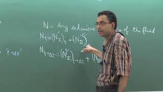
Good morning. Let us start today on boundary layer approximation, the second part. In the last class, we discussed about what is the utility of the boundary layers concept as well as also demonstrated different type of boundary layers. which we generally feel it not flow past an object. Also the mixing layers, the wake formations, jet formations we commonly encounters boundary layers and those boundary layers how we can solve it a part of a approximation solutions of Navier-Stokes equations.
Detailed Explanation
Boundary layers play a crucial role in understanding fluid flow near solid surfaces. The lecture emphasizes that boundary layers are not just limited to flow past solid objects, but also occur in scenarios like mixing layers and jets. We can derive useful approximations using Navier-Stokes equations to analyze these layers. Understanding boundary layers is essential because they determine factors like drag and shear stress, which are critical in engineering applications.
Examples & Analogies
Imagine a car moving through the air. The air closest to the surface of the car moves slower than the air further away. This happens due to the boundary layer effect. If we didn’t understand these layers, we wouldn't be able to design cars that are efficient in terms of aerodynamics.
Computational Tools and Historical Context
Chapter 2 of 6
🔒 Unlock Audio Chapter
Sign up and enroll to access the full audio experience
Chapter Content
These lectures are designed to look at present context is that we have a lot of computational fluid dynamics tools which we can solve the full Navier-Stokes equations. So boundary layers concept here is given as introductory levels to try to understand what is the boundary layers.
Detailed Explanation
The lecture highlights the significant evolution of fluid dynamics analysis from manual approximations to the utilization of computational fluid dynamics (CFD) tools. While boundary layers were once analyzed using handwritten mathematics, modern tools now provide detailed simulations of fluid flow, allowing for precise design and analysis.
Examples & Analogies
Think of how weather forecasting has progressed. Years ago, meteorologists relied on manual calculations of weather patterns. Today, they use sophisticated software that predicts weather with high accuracy, much like how CFD tools allow engineers to predict fluid behaviors efficiently.
Boundary Layer Equations and Assumptions
Chapter 3 of 6
🔒 Unlock Audio Chapter
Sign up and enroll to access the full audio experience
Chapter Content
Today I talk about boundary layer equations which is is a approximations of the basic Navier-Stokes equations. We will discuss it what are the assumptions behind these boundary layers equations that is what we should know it.
Detailed Explanation
This portion introduces the boundary layer equations derived from the Navier-Stokes equations, crucial for understanding fluid behavior near surfaces. Importantly, the assumptions made during this derivation, such as steady flow and neglecting gravitational forces, simplify complex real-world problems into manageable equations.
Examples & Analogies
Consider a doctor diagnosing a patient. To avoid complex medical terminology, they often simplify the diagnosis into terms the patient can understand. In a similar way, engineers simplify the complexity of fluid dynamics to get to the core of the problem.
Understanding Reynolds Numbers
Chapter 4 of 6
🔒 Unlock Audio Chapter
Sign up and enroll to access the full audio experience
Chapter Content
If Reynolds number x is less than 10 to the power 5 that is what 1 lakh. The flow remains in these stretches is laminar natures okay. This is what laminar natures.
Detailed Explanation
Reynolds number is a dimensionless quantity used to predict flow patterns in different fluid flow situations. A Reynolds number below 100,000 indicates laminar flow, where fluid particles move smoothly in parallel layers. Understanding Reynolds numbers is vital for predicting when flow transitions from laminar to turbulent.
Examples & Analogies
Consider a calm river. When water flows slowly, everything is smooth, much like laminar flow. But as the water speeds up, it starts to swirl and create eddies—this represents turbulent flow. The speed at which this occurs can be understood through Reynolds numbers.
Boundary Layer Thickness and Its Significance
Chapter 5 of 6
🔒 Unlock Audio Chapter
Sign up and enroll to access the full audio experience
Chapter Content
What is the thickness of boundary layer thickness as I discussed that this is the thickness what we are defining which is having the velocity the u component close to the 0.99 of free stream velocities.
Detailed Explanation
Boundary layer thickness is defined as the distance from the surface where the flow velocity reaches 99% of the free stream velocity. Recognizing this thickness helps engineers in calculating pressures, drag forces, and the overall performance of objects moving through fluids.
Examples & Analogies
Think of a swimmer diving into a pool. The water closer to the swimmer moves slower than the water further away due to friction—this slow-moving area is similar to the boundary layer around a swimming object.
Applications of Boundary Layer Concepts
Chapter 6 of 6
🔒 Unlock Audio Chapter
Sign up and enroll to access the full audio experience
Chapter Content
We try to avoid the transitional zone by introducing a tripwire. Many of the structures if you look at that they put the tripwires okay which reduce the transitional zones and make it a laminar to transition with a short span.
Detailed Explanation
In engineering, reducing the transitional zone between laminar and turbulent flow can improve performance and reduce drag. One method to achieve this is by adding tripwires that disrupt the boundary layer, helping maintain smoother laminar flow over longer distances.
Examples & Analogies
Picture a runway where planes are taking off. Engineers often streamline the runway surface to ensure planes can take off smoothly. Similarly, tripwires can help manage airflow over surfaces to maintain efficient movement.
Key Concepts
-
Boundary Layer: Critical to understanding how fluids behave near solid surfaces.
-
Reynolds Number: A key factor in determining flow state; lower indicates laminar, higher indicates turbulent.
-
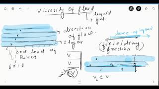
Laminar Flow Characteristics: Smooth and orderly, represented by layers.
-
Turbulent Flow Characteristics: Chaotic flow marked by mixing and eddies.
Examples & Applications
An example of a laminar boundary layer is the smooth flow of water over a flat plate with slow movement, leading to negligible turbulence.
In contrast, the turbulent boundary layer, like that seen in a river's rapids, displays chaotic changes and interactions.
Memory Aids
Interactive tools to help you remember key concepts
Rhymes
In a stream of flow so grand, boundary layers do take a stand. From zero speed on surfaces tight, to free stream's swift, a wondrous sight.
Stories
Once upon a time, there lived a fluid that dreamt of racing down a sloped road. It started slow by a wall, but as it gained speed, its layer grew thin, and the race began!
Memory Tools
Remember 'BLOSSOM' for boundary layers, ‘BRIGHT’ for Reynolds' distinction: below is laminar, rising indicates turbulence.
Acronyms
Use 'VEGA' - Viscosity Eliminated Gravity Approximations for problem-solving boundary layer equations.
Flash Cards
Glossary
- Boundary Layer
The region in a fluid flow where the velocity changes from zero at the surface due to viscosity to almost free stream velocity.
- Reynolds Number
A dimensionless quantity that helps predict flow regimes; it indicates whether flow is laminar (< 10^5) or turbulent (> 3 x 10^6).
- Laminar Flow
A smooth, orderly flow of fluid characterized by layers sliding past one another.
- Turbulent Flow
A chaotic and mixed flow of fluid characterized by irregular fluctuations.
- NoSlip Condition
The condition where fluid velocity at a solid surface is equal to zero.
Reference links
Supplementary resources to enhance your learning experience.